Facies Vectors: Disentangling Environmental Variability, Diagenesis, and Secular Change in Carbonate Stratigraphies

1. Introduction

Stratigraphic signals are a primary mode of inquiry in geology. Since the law of superposition was originally proposed by Steno in 1669 (Steno & Winter, 1916), assembling lithological observations, geochemical measurements, and fossil occurrences in stratigraphic order has been a clear way of organizing the geologic record and formulating hypotheses of environmental change over time. Stratigraphic signals also are especially powerful because they can be used to interrogate a single outcrop or correlated into regional and global compilations such that the scale of observation can match the question at hand. Placing geological data on a timeline in stratigraphic order has led to many foundational discoveries about the nature of Earth history, from identifying Ir anomalies in a few short stratigraphic columns that implicate an extraterrestrial impactor in shaping biodiversity (Alvarez et al., 1980), to the recognition of mass extinctions by compiling global fossil occurrences over the Phanerozoic (Raup & Sepkoski, 1982).

A large portion of well-studied signals come from carbonate stratigraphies, as these archives are abundant (Peters & Husson, 2017), record information relating to both seawater chemistry (Morse & Mackenzie, 1990) and physical environment (Bathurst, 1972) at the time of deposition, and host well-sampled fossil assemblages (Balseiro & Powell, 2023). The information-rich nature of carbonates implies that these rocks can simultaneously host indicators for a broad suite of secular trends in Earth history, like glacioeustasy, 𝛿¹³C values of dissolved inorganic carbon (DIC), and biodiversity. This potential, however, is accompanied by a caveat: these environments are heterogenous and not straightforward recorders of global conditions. Studies of modern carbonate depocenters do not reveal uniform veneers of sediments accumulating across the entire platform (Ginsburg, 1971), but instead show a patchwork of sub-environments with diverse physical, chemical, and biological characteristics (Geyman et al., 2021; Geyman & Maloof, 2021; Harris et al., 2015; Purkis et al., 2012, 2015; Rankey, 2004; Wilkinson & Drummond, 2004). Further, for many key geological metrics, this sub-environmental variability that exists at a single point in time is of equal or greater magnitude as the range of secular change interpreted from the geologic record.

As examples, carbon isotope ratios, which often are leveraged in studying past perturbations to the global carbon cycle and are associated with major events in the coevolution of life and climate, have environmentally-specific signatures (Ingalls et al., 2020), and a variance in sediments on the modern Great Bahama Bank (GBB) that rivals the scale seen in the past two billion years of carbonate stratigraphy (Geyman & Maloof, 2021). Categorical carbonate facies that are used to infer changes in water depth and flow regime, occur across the entire GBB and platforms in the Red Sea without any reliable relationship to either environmental characteristic (Dyer et al., 2018; Geyman et al., 2021; Harris et al., 2015; Purkis et al., 2015). Additionally, organismal distributions can both cause and react to these environmental gradients, and so groups like corals can show species counts that range from < 5 to > 30 along a single spatial transect (Huston, 1985).

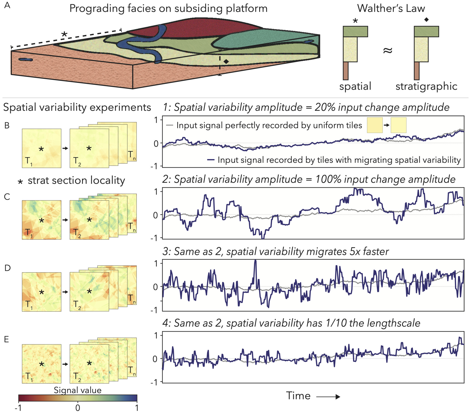
In the absence of secular change, these variable sub-environments migrate laterally due to local processes, like progradation (Burgess, 2001; Ginsburg, 1971), avulsion of tidal channels (Maloof & Grotzinger, 2012), build-up and erosion of islands (Burgess et al., 2001; Burgess & Wright, 2003; Purkis & Harris, 2016), and predominant wind/wave regimes (Neal et al., 2021). As the platform subsides and creates accommodation space for sediments, the sub-environment that exists at one point in space and time eventually will be buried by the next set of depositional conditions to migrate over top (Burgess, 2001; Drummond & Wilkinson, 1993; Geyman et al., 2021; Ginsburg, 1971). The column of sediment that accumulates at a particular point, therefore, represents this environmental migration according to Walther’s Law (Middleton, 1973) and is a stack of depositional conditions that existed contemporaneously, even if preserved over time (fig. 1A; Dyer et al., 2018; Geyman et al., 2021). This interchangeability of space and time, in concert with the extreme heterogeneity of carbonate platforms, requires that some portion of variability seen as stratigraphic signals stems from migrating depositional environments. In fact, because carbonate platforms are as variable as secular changes expected in the geologic record, environmental migration should form the null hypothesis when interpreting a carbonate stratigraphic excursion (fig. 1B–E). In this study, we will evaluate an outcrop starting with this null hypothesis, and only once we constrain the relative contribution of environmental variability, can we interpret broader shifts in the Earth system.

Figure 1.The relationship between spatial variability and secular temporal change. (A) Walther’s Law (Middleton, 1973) gives the expectation that spatial variability in contemporaneous platform environments will be reflected in stratigraphic relationships. As depositional bodies migrate on a subsiding platform, those that are adjacent in space are most likely to be deposited consecutively in the resulting stratigraphy. Using this concept, we can create an illustrative model where various depositional bodies migrate over time while producing a stratigraphic volume, to isolate the effects of spatial variability amplitude (input to the model as a ratio of original signal variability), migration rate, and lengthscale (B–E). (B) In a synthetic experiment, when the amplitude of spatial variability is small relative to the overall amplitude of the input signal, the recorded signal remains relatively faithful to the input. (C) When the amplitude of spatial variability becomes equal to that of the input temporal signal, the record no longer reflects the original input. The vast majority of excursions now stem from the migration of local sources of variability, and it would be challenging to assess which parts of the record accurately reflect the input signal without a priori knowledge of either the input signal, or the sources of variability within the system. (D) When the same sources of spatial variability from (B) migrate 5× faster—equivalent to slowing the platform subsidence rate or accelerating carbonate production—this speeding-up is reflected by shortening of the period for spatial variability excursions. Further, the faster migration means that more of this spatial variability is sampled in an equal amount of time, and so the most extreme cases of spatial variability become more common in the record. (E) When the same experiment from (B) is run with a 1/10 the spatial variability length scale, we also see a shortening of the period for spatial variability excursions. As the sources of variability become spatially smaller, we become less likely to sample extremes at our single stratigraphic locality.

Commonly, geologists will measure parallel sections across a fossil platform and correlate signals to give evidence that an excursion is not a phenomenon of local variability (e.g., Goldhammer et al., 1991; Hillgaertner, 1998; Hofmann, 1977; Husson et al., 2015; Rose et al., 2012). However, the migration of local depositional environments introduces diachronous surfaces that do not necessarily represent a secular event (Dyer et al., 2018; Geyman et al., 2021; Sarg, 1988). In fact, the parallel section approach, especially when large distances >100 km separate localities, often incorporates lateral variability into the correlation model (e.g., Nelson et al., 2023; Smith et al., 2016). Thus, even when correlating across a basin, we still must answer a key question: What is the contribution of the local sub-environment that deposited each bed to the overall trend we see in the stratigraphy? For a detailed discussion of how lateral variability impacts section correlations and subsequent assessments of regional-to-global signals, see the supplementary information section Lateral variability and section correlations.

1.1. Addressing a highly-variable system through lithofacies

Definition note: We will use both the words facies and lithofacies in this manuscript. We mean facies as a more general term to encompass all possible descriptors and categorizations of rock samples that may pull from various observational sources, such as lithology and geochemistry. We use the term lithofacies when specifically referring to either the qualitative or quantitative descriptor of a rock that relies solely on physical lithological properties.

This issue of searching for potentially small secular trends while contending with large internal variability (which we will refer to as having a low signal-to-variability ratio; S:V) is not unique to carbonate stratigraphy. This setup is akin to the modern scientific question of quantifying temperature increases in our changing climate, with the knowledge that fluctuations due to weather and seasons will be much larger than the climate expected signal. At any given locality, temperature changes over the last century may be approximately 1 ^°C, but those expected secular changes are dwarfed by seasonal cycles and weather patterns that give the system a variability that can be >40 ^°C. In climate science, the solution to relieve ambiguity with low S:V is to use well-sampled (both temporally and geographically) records to provide enough context for observations and understanding of the system to ultimately constrain the long-term trend (Hansen et al., 2010). On the other hand, the geologic record is woefully incomplete compared to the past century of climate data, and so we will not be able to constrain stratigraphic signals with this same approach. We can, however, seek to understand the source of ‘weather’ in the stratigraphic record, and use what we learn about the contribution of those factors to a given signal to at least better approximate secular trends.

The conditions of the local sub-environment at the time of deposition of each bed likely are the primary source of non-secular variability in carbonate stratigraphies. As geologists, we already use lithological observations as a framework for describing paleoenvironment in a set of strata. The where and how of sediment deposition on a platform often are read from physical rock characteristics like grain sizes and abundances, as well as bedforms. The main hurdle in directly applying this existing framework to better understand signals is the fact that the metrics that constrain sub-environmental variability on modern platforms often are more quantitative and nuanced than traditional lithology categories. For example, a major factor contributing to lateral changes in 𝛿¹³C values on the GBB is the exact proportion of different carbonate sediment types in a sample (Geyman & Maloof, 2021). And so, a typical note like ‘sparse shells’ or ‘abundant ooids’ that may accompany a 𝛿¹³C value likely does not contain enough fine-scale information to capture the sub-environmental context contributing to that measurement.

Additionally, unlike fossil occurrences and chemical data, qualitative lithology assessments are not numerical. So, while we can model and make quantitative inference between biodiversity and inferred ocean chemistry, we do not have scaling factors that link qualitative lithology to numbers that can be analyzed alongside other metrics. This lack of numerical translation, even for semi-quantitative notes like ichnofabric index (Bottjer & Droser, 1991), or depth rank (Olsen, 1986), is further hindered by lithological observations being specific to the particular geologist that recorded them. Scientists incorporate hunches that influence the compilation and visualization of data (Lin et al., 2023), such as how a stratigrapher may make observations in light of which surfaces they think represent the tops of parasequences (Dyer & Maloof, 2015). In geology, these hunches are not just scientist specific, but have evolved over time as guiding biases changed through paradigmatic shifts like the understanding that shifting ice volumes can produce large eustatic changes (Wanless & Shepard, 1936), or the introduction of plate tectonics (Dickinson, 1974). Without reproducible methods to return to, we likely cannot disentangle the hunches of each geologist and era to find reliable relationships between an assessment of ‘ichnofabric index 4’ or ‘very coarse grainstone’ and chemical or biodiversity data. Therefore, to understand the influence of depositional conditions on carbonate stratigraphic signals, we need lithofacies observations that are fully quantitative, reproducible, and readily pair with chemical and fossil occurrence data in integrated models and cannot be reproduced or included across meta-analyses.

Post-burial diagenesis also impacts stratigraphic trends in geochemical variables (Ahm et al., 2018; Higgins et al., 2018), biodiversity (Behrensmeyer et al., 2000; Kidwell et al., 2005), and hydrological indicators (Coogan & Manus, 1975). These effects can be both facies dependent and independent, and also act to lower S:V in carbonate stratigraphies. In our supplementary materials section Diagenesis, we briefly survey some background literature on the topic, and we keep this influence of diagenesis in mind throughout the study.

1.2. Cambrian case study

While lithofacies and diagenesis serve to give carbonate systems low S:V, we can use modern analogs as a guide to define tests for identifying and quantifying these sources of variability, and constrain the proportion of a signal that is attributable to secular environmental change. In this study, we develop methods that allow us to quantitatively investigate at this intersection of lithofacies, diagenesis, and environmental change, and apply them to a lower Cambrian outcrop.

We specifically choose this period because the early Cambrian (Terreneuvian and Epoch 2; 539 to 509 million years ago) is a time classically investigated for secular trends that may relate to the rapid evolutionary change seen in early metazoans. For additional motivation to investigate lithofacies effects on Cambrian signals, see our supplementary materials section Correlations between qualitative lithofacies and 𝛿¹³C values in an extended lower Cambrian record. Within this relatively short interval, nearly all animal phyla recognized today first appear in the fossil record (Valentine, 1995), skeletonized species and genera become abundant and diverse (Erwin & Valentine, 2012; Lipps & Signor, 2013; Zhuravlev & Riding, 2001), and metazoan community structures begin to appear ecologically similar to the modern day (Erwin & Valentine, 2012). These events are clear landmarks in the history of life on Earth, and so the early Cambrian is the subject of many studies seeking to constrain causal explanations.

Whether giving evidence of a proposed environmental trigger, like increased oxygenation (Berkner & Marshall, 1965; Canfield et al., 2007; Catling et al., 2005; Dahl et al., 2019), or the response of Earth systems to new animal behaviors, like the rise of burrowing life modes (Bottjer et al., 2000), early Cambrian research often relies upon stratigraphic signals—such as the record of 𝛿¹³C values from supplementary figure 2. This methodology is used at multiple scales, from measured sections looking for environmental change within a single Cambrian outcrop or basin, to global proxy compilations (Peng et al., 2020). On the local-to-regional scale, many recent studies have accompanied measured sections with carbon cycle (𝛿¹³C values, total organic carbon) and redox proxies (iron speciation, 𝛿³⁴S values, Mo and other trace metal concentrations) that show some intrabasinal correlations between interpreted oxygenated bottom waters, carbon cycle perturbations, and fossil occurrences (He et al., 2019; Wei et al., 2018). Global compilations of lower Cambrian stratigraphies also identify the interval as one of possible geochemical overturn, presenting signals that correlate across basins and contribute to the hypothesis of oxygenation through either carbon or sulfur cycle systematics (Betts et al., 2018; Dahl et al., 2019; Maloof et al., 2010; Smith et al., 2016). On an even larger scale, datasets that comprise global proxy records and models that cover geologic eras and eons find indications of unique marine conditions in the Cambrian. Most notably, these studies have pointed out a possible rise in atmospheric oxygen near the Precambrian–Cambrian boundary (Lyons et al., 2014), as well as a Cambrian peak in shallow continental shelf area and nutrient delivery to the ocean (Brasier & Lindsay, 2000; Peters & Gaines, 2012; Tasistro-Hart & Macdonald, 2023).

Figure 2.Motivation for non-stratigraphic study methods to constrain the relative impacts of reef environments to ancient ecosystems and biodiversity. (A) Data from Idjadi and Edmunds (2006). In modern, shallow-water tropical environments, there is a well-documented relationship between the amount of topographic complexity or roughness imparted to the seafloor by coral reefs and the number of invertebrate genera that live nearby (Idjadi & Edmunds, 2006; Kostylev et al., 2005). (B) In a previous study, Manzuk et al. (2023) showed that early Cambrian archaeocyaths had similar roughness measurements to modern, biodiversity-building Scleractinian corals, and much higher than stromatolites that would have built reefs in the Precambrian. (C) These data indicate that the rise of reefs could have been a major influence on Cambrian biodiversity, but further investigations into that relationship cannot take place through stratigraphic signals for two main reasons. Reefs are a relatively small portion of carbonate platforms (Geyman & Maloof, 2021; Purdy & Gischler, 2003) that may have an outsized environmental influence, and so the conclusion from figure 1 that small length scale sources of unique variability often evade a single stratigraphic section applies to reefs. Reefs themselves also are highly heterogenous, and so assigning a single value to them as a bed for any metric under constrains them as a paleoenvironment.

With this abundance of literature concerning the early Cambrian, we have numerous scales and environmental proxies to begin investigating the relative influence of lithofacies and diagenesis on an interpreted signal. We choose in this study to work on a single stratigraphic section. As regional and global studies compile chemical data and fossil occurrences that stem from single outcrops, we first need to understand the caveats that underlie observations and interpretations at this small scale before we can prognosticate broader outcomes. For additional motivation regarding an in-depth look at the stratigraphic trends from a single outcrop with implications for the global Cambrian, see the supplementary information section Correlations between qualitative lithofacies and 𝛿¹³C values in an extended lower Cambrian record.

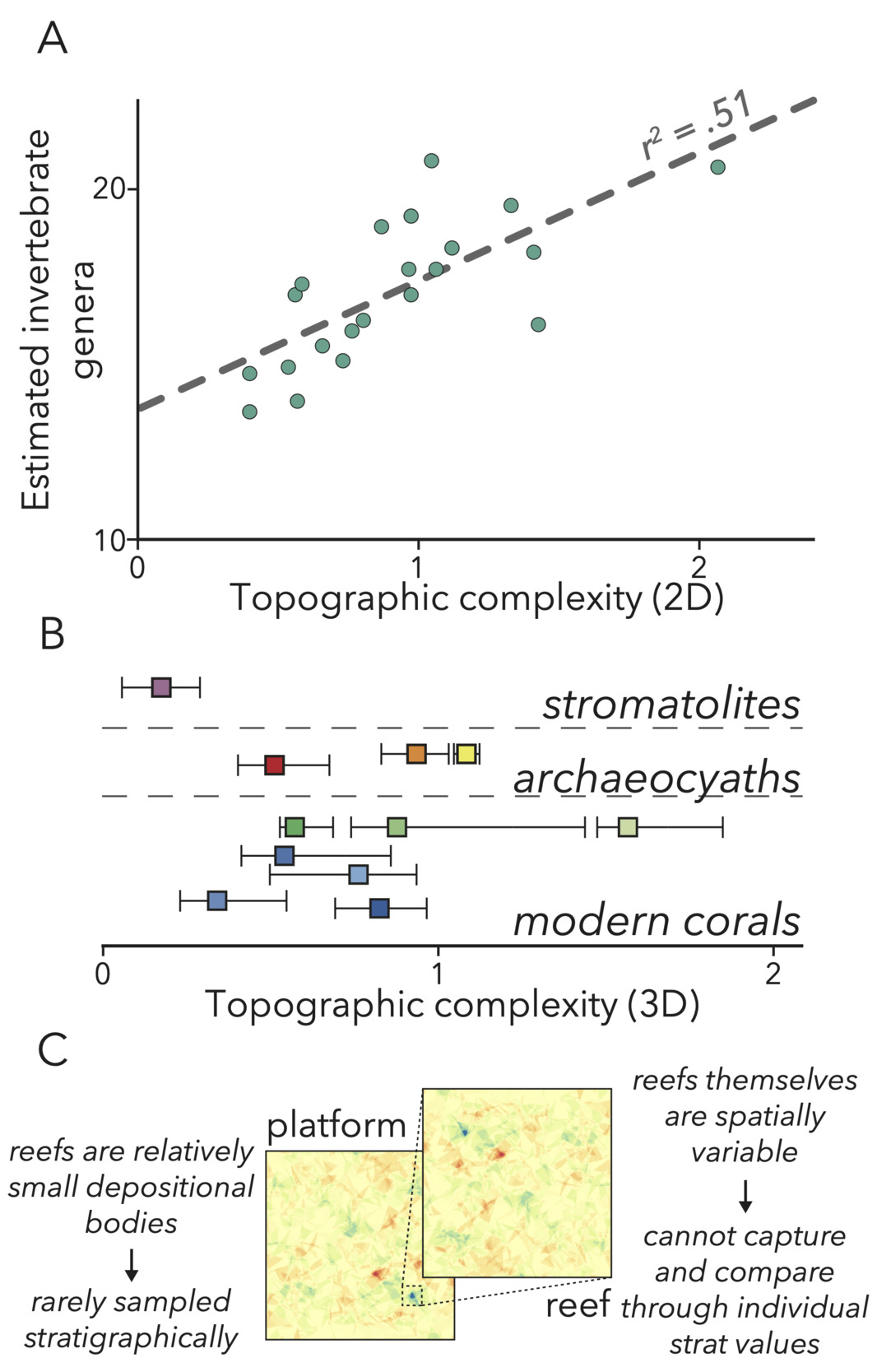
This outcrop allows us to investigate a component of Cambrian platforms that may have contributed to biodiversification at the time but is difficult to study in a stratigraphic approach. Specifically, we look to further constrain the environmental engineering impact of Earth’s first framework reefs, built by archaeocyaths—a group of extinct, heavily-calcifying sponges (Debrenne, 2007; Pratt et al., 2000). Reefs are a crucial element of modern marine environments (Idjadi & Edmunds, 2006), as the rough (fig. 2A, B) and massive structures built by Scleractinian corals provide both physical spaces (Kostylev et al., 2005) and modified fluid dynamics (Monismith, 2007) in shallow environments to promote the development of diverse and abundant metazoan communities. Although these important environments are found in outcrops covering the entire Phanerozoic (Kiessling, 2002), reefs rarely are implicated as factors in ancient biodiversity. Reefs have relatively low likelihood of being sampled at outcrop, both due to their narrow extent (Geyman & Maloof, 2021; James & Mountjoy, 1983; Purdy & Gischler, 2003) and low preservation potential of platform margins (James & Mountjoy, 1983), and so apparent trends in factors such as reef size or abundance may not encapsulate their ultimate impacts on past shallow-water environments. Further, reefs and their surrounding sediments are more heterogenous than other carbonate depositional bodies (fig. 2C), and so capturing reefs with single geochemical or geophysical values in a stratigraphic approach likely does not adequately depict their paleoenvironmental influence. Therefore, our goal in this study is to outline quantitative methods that both alleviate low S:V ambiguities present in all stratigraphies, and unlock the potential to investigate new environmental hypotheses in the evolution of early animals.

2. Materials and methods

2.1. Geological setting and stratigraphic trends

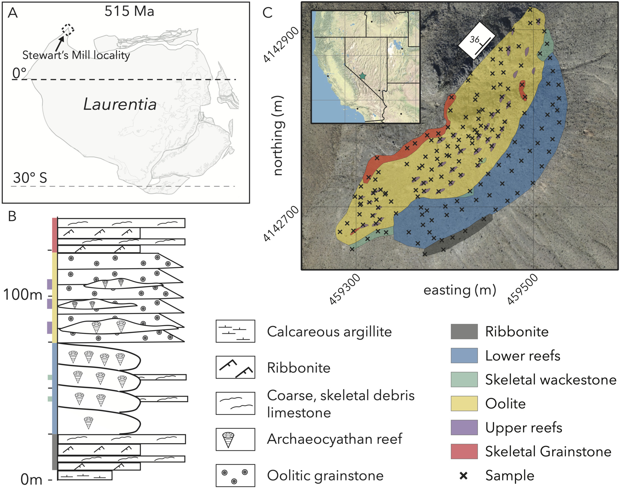
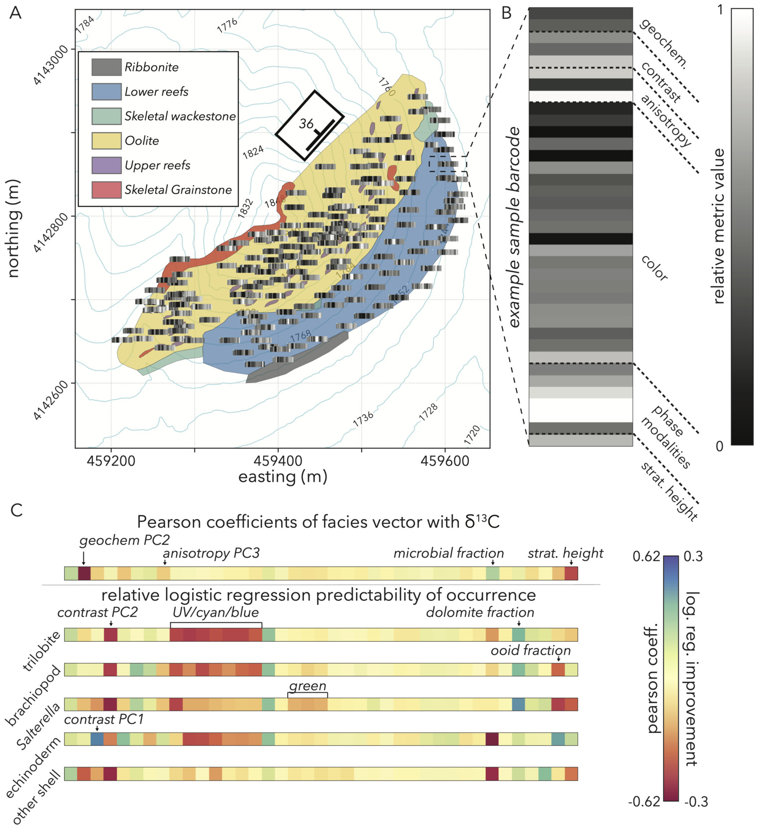
Our study site is a section of the carbonate-rich lower member of the Poleta Formation (Fm), exposed at a locality commonly referred to as Stewart’s Mill (fig. 3A; GPS: 37.430970, -117.458792, WGS84; Rowland, 1984; Rowland & Gangloff, 1988). The Poleta Fm at Stewart’s Mill dips 35^∘ to the northwest and starts with 20 m of bedded carbonate mudstones with occasional interbedded skeletal packstones at its base (fig. 3B). Above the bedded interval are approximately 50 m of reef complex (Rowland et al., 2008) with massive boundstones dominated by the calcimicrobial taxon, Renalcis. The lowest reefs contain few (∼3% estimated volume) archaeocyaths of diverse morphologies and gradually increase in abundance towards the top of the interval (up to 13% estimated volume Rowland & Gangloff, 1988). In this lower complex, reef flanks occasionally are draped with argillites with interbedded skeletal grainstones (fig. 3B). Above these more microbe-dominated reefs, the section transitions into ∼40 m of coarse oolitic grainstone and skeletal grainstone interbeds with oolite intraclasts (fig. 3B). The lower 20 m of this oolitic interval shows occasional dune-scale cross-stratification and contains 3–5 m-wide, 1–2 m-high archaeocyathan patch reefs. These reefs mostly contain two genera (Paranacyathus and Protopharetra), which show branching morphologies in the field (Rowland & Gangloff, 1988). Three-dimensional morphological measurements of these archaeocyaths show that these branching structures are nearly identical to photosynthetic corals building biodiverse reefs in the modern (Manzuk et al., 2023). Overall, this section contains a diverse suite of microbial and metazoan reefs, along with their attendant environments. This variety of carbonate lithologies, closely associated within a small, ∼30,000 m² area of exposure provides an ideal study system to test relationships between lithofacies, chemical signatures, and fossil occurrences.

Previous authors have recognized geochemical and ecological stratigraphic trends at Stewart’s Mill. While we will not explicitly test our results against any prior conclusions of change through time at this outcrop, preferring to focus on the general null hypothesis of carbonate environmental variability as a source of stratigraphic signals, these studies provide a useful set of stratigraphic expectations. Three authors have produced similar records of 𝛿¹³C values for the reef-bearing member of the Poleta Formation, where the values trend linearly from ∼0.5‰ at the bottom of the section to ∼-1.5‰ at the top (Cordie et al., 2019; Pruss & Clemente, 2011; Rowland et al., 2008). This gradual 2‰ downturn in a relatively short section is difficult to correlate to any global compilations and is not interpreted to represent large-scale carbon cycle overturn hypothesized with respect to other lower Cambrian signals (Rowland et al., 2008). Ecologically, the reefs are hypothesized to progress from a colonization phase to a diversification stage, and finally a dominance or foundering stage (Pruss & Clemente, 2011; Rowland, 1984; Rowland et al., 2008). Throughout this progression, archaeocyath abundance and contribution increase greatly within reefs (Cordie et al., 2019; Pruss & Clemente, 2011; Rowland, 1984), but the trends in other metazoans remain uncertain (Cordie et al., 2019). Identified ecological affinities by animal communities for certain reef phases (Pruss & Clemente, 2011) question whether diversity on this carbonate platform goes through any changes through time, or if trends can be explained by the null hypothesis of sub-environmental variability.

Figure 3.Geological setting and field methods. (A) A Laurentian paleocontinent reconstruction after Torsvik and Cocks (2016) and Domeier (2018) places the Stewart’s Mill study location within the northern hemisphere tropics. (B) Generalized stratigraphic column of the Stewart’s Mill study site, see main text for discussion. (C) Our drone-derived imagery, combined with our grid-based approach for mapping observations and samples yields a high-resolution geospatial dataset for further investigations of local trends in depositional setting, diagenesis, and environmental change.

2.2. Field methods

To produce a base map of the field site at Stewart’s Mill (fig. 3C), we captured aerial imagery with a senseFly eBee fixed-wing drone with original resolution of under 4 cm per pixel and stitched the images into an orthomosaic with Agisoft Metashape software. We georeferenced the orthophoto base map by placing four 1.2 × 1.8 m blue tarps in the zone captured by the drone-derived photographs and constrained the corner locations of each tarp with a Trimble GeoXH Rover differential GPS (dGPS) unit (<0.2 m uncertainty).

After measuring a stratigraphic section (fig. 3B) to constrain basic lithologic relationships and qualitative lithofacies groups, we walked an approximate grid with ∼10 m spacing to map the outcrop. At each point on the grid (fig. 3C), we marked the location with a dGPS point, made observational notes,—including the orientation of bedding and cleavage planes, sedimentological observations, and qualitative carbonate lithofacies characterizations—and collected a fist-sized sample. Prior to extracting samples, we measured and marked the strike and dip of the most planar exposed face to preserve sample orientation for later reference.

2.3. Quantifying lithofacies

Our goal is to capture the properties of rock samples that a geologist can see and uses to make lithologic categorizations, and translate these characteristics into reproducible quantities that easily can be used for pattern finding and model building. Our basis for assessing these quantities are petrographic images of polished slabs from each sampled point in our map grid, upon which we perform image analyses. We prepare these slabs in a semiautomated routine with the Grinding, Imaging and Reconstruction Instrument at Princeton University (Mehra et al., 2022) and capture petrographic images with the multispectral imager described in Manzuk et al. (2022) at a spatial resolution of 3.76 𝜇m per pixel. Details on the sample preparation and imaging process can be found in our supplementary materials section Polished slab preparation and imaging.

With quality petrographic images for all samples, we now can create algorithms to reproducibly and quantitatively describe lithofacies characteristics to understand the influence of depositional environment on signals at our study outcrop.

2.3.1. Sample texture

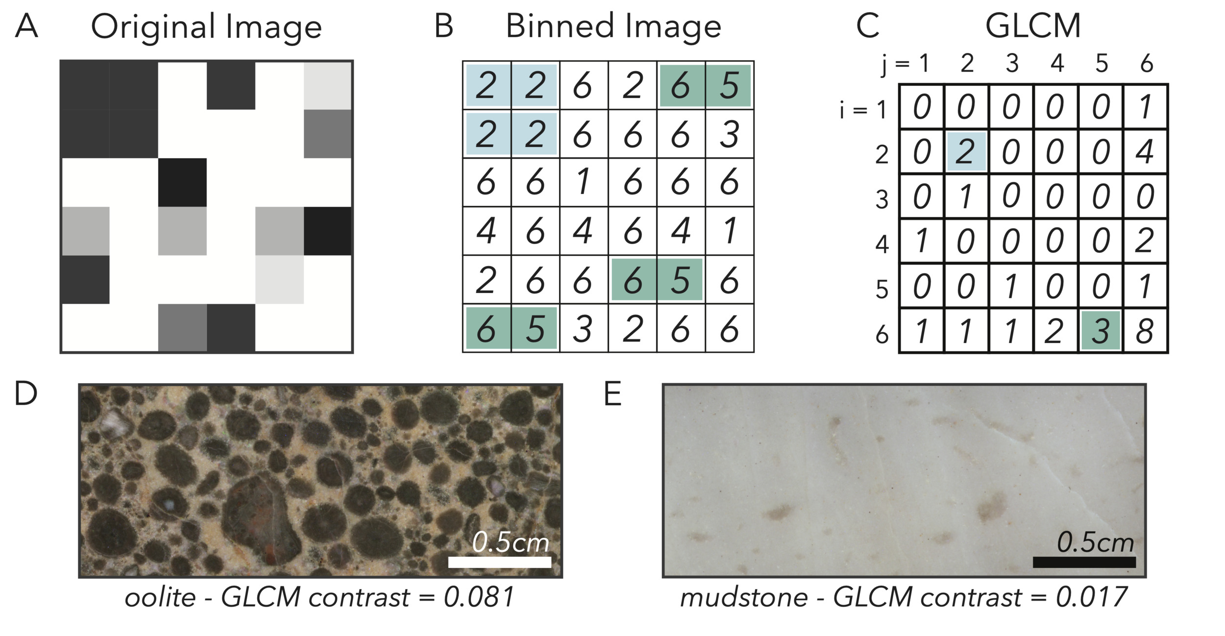
We want to capture the relatively high-contrast or homogenous appearance of samples that relates to lithofacies. For example, a heterogenous fine grainstone will show a large amount of fine-scale contrast as transitions between adjacent pixels may capture sharp boundaries between differently-colored grains (fig. 4D), whereas a carbonate mudstone may appear as uniform gray (fig. 4E). To build intuition for quantifying these textures, we can think of each image as an elevation model of a landscape. The height at each point is given by the pixel intensity, and so relatively bright pixels will be high, and relatively dark pixels will be low. In this model, heterogenous areas with fine-scale transitions between light and dark will look like a jagged mountain range, and homogenous areas where color intensity smoothly transitions (or does not change) will appear as plains and rolling hills.

Figure 4.Texture assessment through gray level co-occurrence (GLCM) contrast. (A, B) We bin grayscale images based upon pixel intensity into a defined number of gray levels. We show six gray levels here for compactness, but we use eight in full analyses, as is typical practice with GLCMs. (C) The GLCM is a square matrix that results from counting the total number of occurrences of a pixel binned to the 𝑖th level occurring next to a pixel binned to the 𝑗th level. (D, E) When we calculate contrast with equation (1), we find that an oolitic packstone has higher contrast (more textured) than a mudstone, matching the expectation we get when looking at samples with our eyes.

To capture these discrepancies in texture, we use a gray level co-occurrence matrix (GLCM; Haralick et al., 1973) and its resulting statistics. This technique takes a sample image and bins the pixels by brightness with the number of evenly-spaced bins defined by the user (fig. 4A, B; we use the standard eight when analyzing samples). We can think of this step as discretizing our elevation model into a set of steps with eight evenly-spaced heights. The GLCM then is assembled by looking at the association between each pixel and the one on the right (or whichever direction defined by the user). The GLCM is a square matrix of equal dimensions to the number of bins, and each cell contains the total number of occurrences of a pixel binned to the 𝑖th level occurring next to a pixel binned to the 𝑗th level (fig. 4C). Relatively homogenous images will be represented by GLCMs with counts mostly distributed along the diagonal, as pixels will tend to have similar intensities to those adjacent. High contrast images will have GLCMs distributed more towards the lower-left and upper-right corners, away from the diagonal. Of the possible GLCM statistics, we find the most informative to be contrast, which is defined as:

\[\begin{array}{r} contrast = \ \sum|i - j|^{2}p(i,j),\tag{1} \end{array}\]

Where 𝑖 and 𝑗 are the row and column index within the GLCM, respectively, and 𝑝(𝑖,𝑗) refers to the proportion of all GLCM counts that fall within the cell at 𝑖, 𝑗.

2.3.2. Sample anisotropy

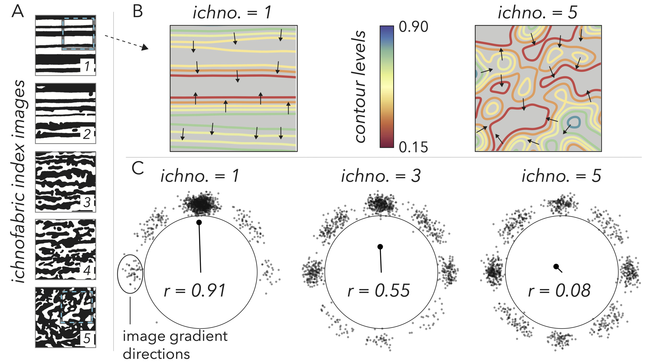
Certain textural features, like bedding and imbrication, are aligned and will give sample images anisotropy. We quantify these features using the image gradient. Returning to the visual of images as elevation models, the gradient at each point in the image is a measure of the surface slope, both in magnitude and direction. As a landscape, a highly anisotropic image will have a series of consecutive, parallel ridges and cliffs that point most of the gradient observations in a similar direction (fig. 5B). To put a number on this alignment in our images, we track the average directionality of the gradient, and not its magnitude such that our measure of anisotropy strictly speaks to alignment of features and remains agnostic as to their brightness or darkness. Our metric is inspired by the Rayleigh Z test (Mardia, 1975), and we start by taking the entire population of gradient headings in an image and force them into the first two quadrants such that upward and downward slopes that are aligned appear as equal angles. We then double all angles to populate the entire unit circle and convert the directions from polar to cartesian coordinates where each measure is given a radius of one (fig. 5C). To get a measure of anisotropy, we take the mean 𝑋 and 𝑌 coordinates of the population and convert this average back to polar coordinates, where the radius of this coordinate gives a measure of alignment. If the gradient directions are completely unaligned and pulled from a uniform distribution around the unit circle, the average position should be near the origin, yielding a radius near zero (fig. 5C). A completely anisotropic image with gradients (forced into the first two quadrants and doubled) all pointing in a similar direction will pull the average position towards the main cluster of angles, giving a radius closer to one (fig. 5C). This radius, our anisotropy metric, is given by the equation:

\[\begin{array}{r} r = \ \sqrt{\left( \frac{\sum{\sin\theta_{i}}}{n_{\theta}} \right)^{2} + \left( \frac{\sum{\cos\theta_{i}}}{n_{\theta}} \right)^{2}},\tag{2} \end{array}\]

where 𝜃_𝑖 refers to the population of gradient angle directions, and 𝑛_𝜃 is the total number of gradient directions in the population from an image (equal to the number of pixels).

Figure 5.Intuition for quantifying anisotropy in sample images. (A) Ichnofabric images from Bottjer and Droser (1991) provide a test set for quantifying anisotropy in images where the appearance of linear fabrics decreases as ichnofabric index increases. (B) Contour plots of the inset sections of ichnofabric 1 and 5 images illustrate the decrease in anisotropy with increasing ichnofabric index. The index 1 plot shows a set of parallel contours and gradients (small black arrows), whereas the index 5 plot has much more uniformly distributed angles for contours and gradients. (C) To quantify this difference in anisotropy, we place the population of gradient directions from each image around a unit circle (jitter added for clarity), and take the mean 𝑥 and 𝑦 position. The distance of this mean position from the origin assesses the level of anisotropy in the image, where a population of angles with a preferential direction will have a larger radial distance, and a more uniform population will have a mean position closer to the origin. Our metric applied to the ichnofabric images gives the anticipated result of decreasing anisotropy with increasing ichnofabric index.

2.3.3. Phase modalities

We assign phase modalities through point counting using the JMicroVision (v1.3.4) software (Roduit, 2010). Point counting is an often-used technique in paleontology and petrography where a grid or random assortment of points is stepped through on a sample, and each point is labeled with the corresponding phase present at that location (Gibbon & Wyllie, 1969; Harlov et al., 1998; Johnsson & Meade, 1990; McSween Jr, 1977; Nesbitt et al., 1996; Payne et al., 2006; Pruss & Clemente, 2011; Sanderson, 1974). Although this method is an incomplete sampling of the rock surface, and can have biases (Solomon, 1963; Van der Plas & Tobi, 1965), point counting still provides an appropriate first-order approximation of phase modality. The recent rise of artificial intelligence (AI) models for image segmentation (Minaee et al., 2022) may soon facilitate fully automated identifications of all pixels in a petrographic image, offering a complete sampling. However, highly-specific domains like geology will be some of the last fields to get accurate networks that can match detailed human identifications (Brenskelle et al., 2020; Panigrahi et al., 2023; Santos et al., 2020; Wang et al., 2021), and so point counting offers the best phase modality option at this moment.

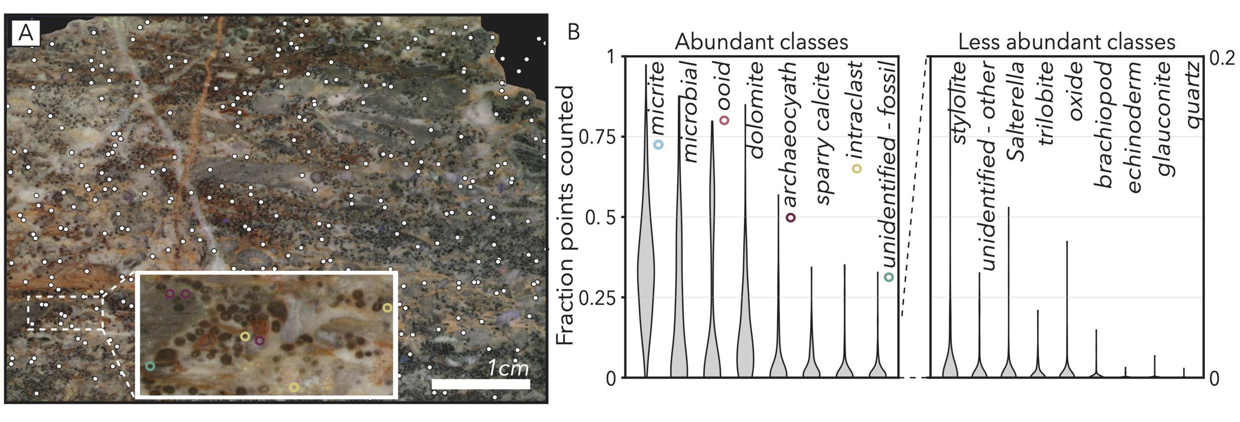
We specifically look to limit biases in our point counting results by opting for random dispersal of our 350 points counted (fig. 6A) such that regularly bedded or graded phases would not be disproportionately sampled if occurring at a harmonic with grid spacings. We also focus our final statistical analyses on the most voluminous classes (micrite, microbial, ooid, dolomite, archaeocyath, spar; fig. 6B). We exclude low volume fraction classes that are small and/or infrequent from final analyses (fig. 6B) because the variance seen in modality data for these phases is more likely to be a product of stochasticity of sampling as opposed to true variance in abundance (Solomon, 1963), especially when approximating three-dimensional elements through two-dimensional cross-sections (Howes et al., 2021; Manzuk et al., 2022; Mehra et al., 2022).

Aside from archaeocyaths, all fossil groups are in this set of classes that is infrequently sampled (fig. 6B). Because we do not have a high-confidence method to assess fossil abundance, but still would like to study biodiversity trends within our sample set, we represent trilobites, brachiopods, echinoderms, Salterella, and unidentified shells simply with presence or absence in our final facies vector. This approach is common in paleobiology, especially when abundance data may suffer from uneven sampling (e.g., Bottjer et al., 1988; Jackson, 2012), and still allows for assessment of trends in coexistence (Mosbrugger & Utescher, 1997). We deem a fossil to be present if it has at least one point counted, and bolster these occurrences by double checking each sample for instances of fossils that were missed by point counting.

Figure 6.Point counting methods to measure phase modalities. (A) On each sample image, we manually assign classes to 350 randomly dispersed points. (B) Classes indicated with colored circles correspond to the points in the inset from (A). In our entire point counted dataset, we note that five classes—micrite, microbial, ooid, dolomite, and archaeocyath—are most abundant and have non-exponential distributions. We use these classes for further statistical analyses as we have the most confidence that the incomplete sampling provided by point counting still accurately represents their volume fraction. Less abundant classes that we still would like to include in further analyses, like fossil groups, we represent as either being present or absent in a sample.

2.4. Lithofacies metric spectra

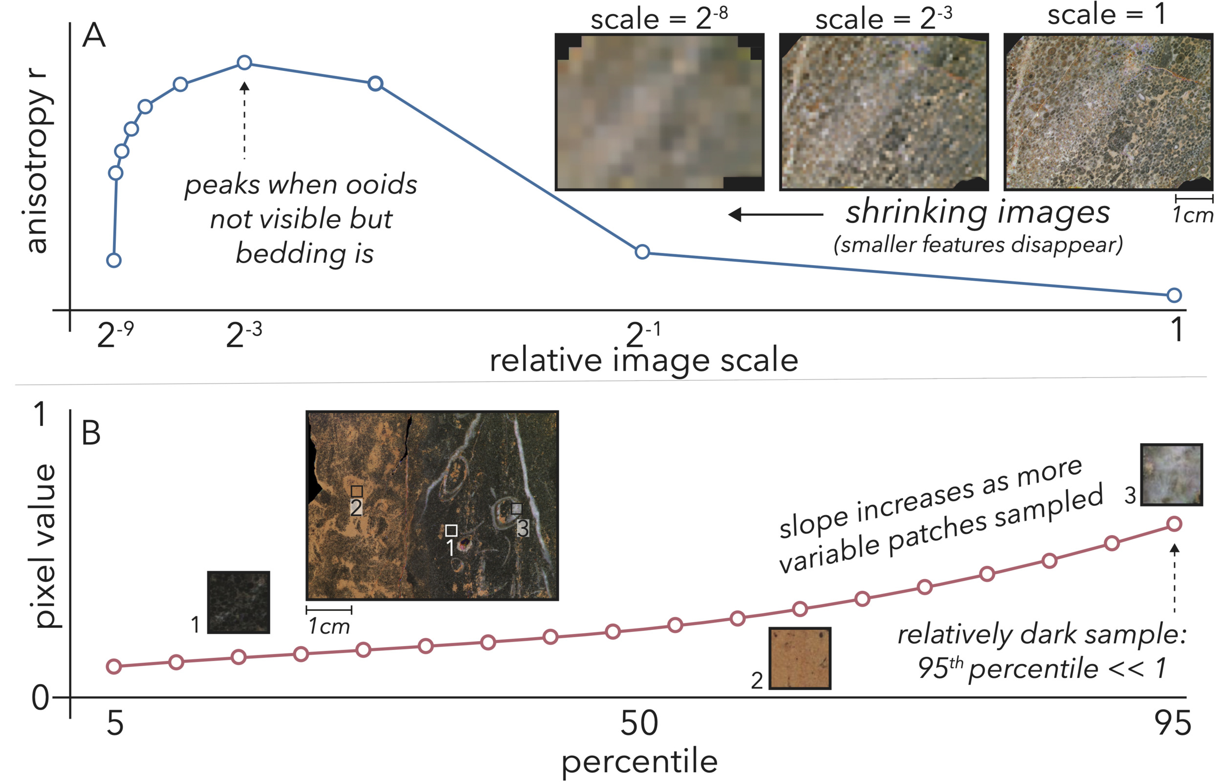
Compared to all the information available in a petrographic image, our color and texture metrics are relatively coarse. Notably for anisotropy and GLCM contrast, we want to have a concept of the sizes of the features that are contributing to a given metric in order to encapsulate factors like scale of bedding or grain size. To that end, we assess our contrast and anisotropy metrics over size spectra starting with the full resolution image. We then repeatedly reduce the image resolution by half until it is 2⁻⁹ scale—at which point it is only 25 x 33 pixels—assessing the metric at each step (fig. 7A). This spectrum then contains information both about the overall texture of a sample, as well as the scale at which it most or least expresses that texture based upon the sizes of its features (fig. 7A). As the image shrinks to smaller scales, coarser features are emphasized as fine features are obscured and removed through downsampling. Thus, these spectra should be interpreted with the inverted logic that smaller scales indicate an emphasis on coarser features causing contrast or anisotropy and vice versa.

In the interest of gathering more spectral information than the mean value for each wavelength, we also assign color as spectra. These color spectra are not based upon scale (as mean spectral signature will not change as the image is downsampled), but instead percentiles of pixel values. Specifically, for each wavelength, we assess every 5th percentile from 5–95, and these values form a spectrum (fig. 7B). Similar to the texture spectra, these color spectra contain information about the overall reflectivity of a sample for a given wavelength, in addition to particulars like if a sample is an even mix of dark and bright elements versus a more homogenous blend of more moderately-reflective components.

Figure 7.Examples of a lithofacies metric spectra. (A) As an anisotropy example, we show a sample image of a graded oolite that has some faint bedding. As we shrink the image (making features relatively blurry) the ooids disappear, leaving the bedding most prominent. Because ooids are a relatively isotropic feature, the size where ooids just disappear but bedding is left prominent, one-eighth scale, gives the relative peak in our anisotropy metric for this sample. Assessing metrics over this spectrum of sizes allows us to encode information about relative feature sizes into our facies vector. (B) We use the 590 nm channel of a dark, dolomitized sample to build intuition for interpreting color spectra. Average image color values would not change with shrinking image scales like in (A), so to get more nuanced color measures, we look at how pixel values are distributed within the full-scale image. For this spectrum, the absolute pixel values will indicate how bright or dark the image is, and the slope of the curve relates to spread or homogeneity in the distribution of pixel values. As an example, a homogenous gray or yellow image would have a spectrum that is a perfectly horizontal line over all percentiles with a pixel value matching the sample brightness. In the sample shown here, the near flat line at low pixel values from 5–50% is a reflection of the majority of the sample consisting of homogenously-dark ooids. The rest of the spectrum has a higher derivative as the pixel value distribution spreads out and more variable dolomite and sparry calcite patches are sampled. Overall, this sample is relatively dark, and so its spectrum maintains values well below the maximum of 1.

2.5. Quantifying geochemical facies

Prior literature about the variability of geochemical observations, especially 𝛿¹³C values, indicates that the primary source of heterogeneity in modern carbonate environments is due to the differing distributions of isotope ratios among different classes of carbonate grains (Geyman & Maloof, 2021; Ingalls et al., 2020). For example, on the GBB, an oolitic grainstone should be expected to have a 𝛿¹³C value of ∼5‰, while a coral rudstone may be at ∼-3‰. These exact grain-associated anomalies of chemical values that we see in modern environments likely are not perfectly replicated in rock samples, but observations like those on the GBB give the intuition that different grain types formed in different locations and conditions may be a primary source of chemical variability in deep time. Additionally, the presence of clearly altered phases like sparry calcite, calcite veins, and dolomitized mud may be indicators of diagenesis. Due to this expectation that carbonate phases should be a main driver of geochemical variability, when drilling powders from our samples for chemical analyses, we first identify all phases present in our sample set that we can reliably identify and extract at least ∼10 mg with a 0.5 mm-diameter bit. Because of the class size limitation for chemical sampling, our phase list for geochemical analyses is modified from point counting and comprises ooid, micrite, sparry recrystallized micrite, dolomitized micrite, calcite vein, archaeocyath, microbial texture, and other fossil shells.

We measure 𝛿¹³C and 𝛿¹⁸O values, as well as elemental concentrations with methods (Edmonsond et al., 2024; Geyman et al., 2022; Geyman & Maloof, 2021) detailed in our supplementary materials section Geochemical measurements.

2.6. Dimension reduction

With both lithofacies and geochemical facies metrics, our raw facies vector contains over 200 parameters per sample, which is too many data to sort through in search of patterns in the relationships between lithofacies, diagenesis, and environmental change. Additionally, color makes up 160 of the parameters, and so there is an uneven emphasis on certain characteristics in the raw facies vector. To decrease this relative emphasis on color, and focus our study on overall fewer, targeted metrics, we reduce dimensionality through principal components analysis (PCA; Wold et al., 1987). This technique takes a multi-variate dataset, performs a singular value decomposition (SVD), and reprojects the original data onto new axes that are orthogonal linear combinations of the original axes. In the resulting principal component (PC) space, the first few axes likely will capture the majority of variance in the dataset, allowing us to study most of the information contained in the facies vector on a much more manageable number of dimensions. We perform a PCA on color, contrast, anisotropy, phase modalities, and geochemical data separately, and represent each of these categories as its most significant PCs in our final facies vector.

3. Results and discussion

This study is focused on the need to understand the influence of depositional environment on stratigraphic signals in chemical metrics and fossil occurrences. With that motivation, we outline some intuitive methods that capture characteristics of depositional environment, such as the nature of bedding and the color, modality, and textural arrangement of granular components. These methods turn petrographic observations into a set of numbers that can be part of a quantitative analysis of an outcrop that operates at the intersection of local depositional environment, diagenesis, and regional-to-global conditions. For our results, we will first build intuition as to how our reduced-dimension facies vector components inform us about the petrographic and geochemical properties of our sample set. We share these dimension reductions as results because they are novel quantitative descriptors of rocks that serve both the current study, as well as to inspire use in future reproducible geologic studies. Then, we will take that foundation and simultaneously analyze the ensemble of facies vector components to build a wholistic picture of the history captured in our outcrop, and discover what this new approach teaches us about the early Cambrian.

3.1. Dimension reductions: the final facies vector components

Here we give a brief outline of the results when reducing dimensions through PCA in each metric category, accompanied by example images that show the types of qualitative observations and interpretations represented by our quantitative facies vector. To keep the discussion brief, our examples mostly emphasize samples that have the highest scores in each PC to show positive examples of the features highlighted by our facies vector. Although not discussed often here, low or moderate scores also are important to our final analysis as indicators of samples lacking features. For each PC, we list the percentage of variance it explains in the dataset to give an idea of the amount of available information encoded in our lithofacies metrics after reducing dimensions. However, we are not implying any association between a PC’s percentage of variance explained and its relative interpretive power or importance in later analyses. Even a small percentage of variance, if related to a key diagnostic feature, such as grain size, still may be a key component in understanding stratigraphic signals.

3.1.1. Spectral signatures

To reduce dimensions of our color percentile spectra, we perform a PCA on each wavelength individually. Additionally, we do not normalize these data prior to the PCA because our color correction practices (see supplementary information subsection Sample spectral signature) should standardize color across samples, and so any remaining variance depicts real and relevant differences in sample reflectance.

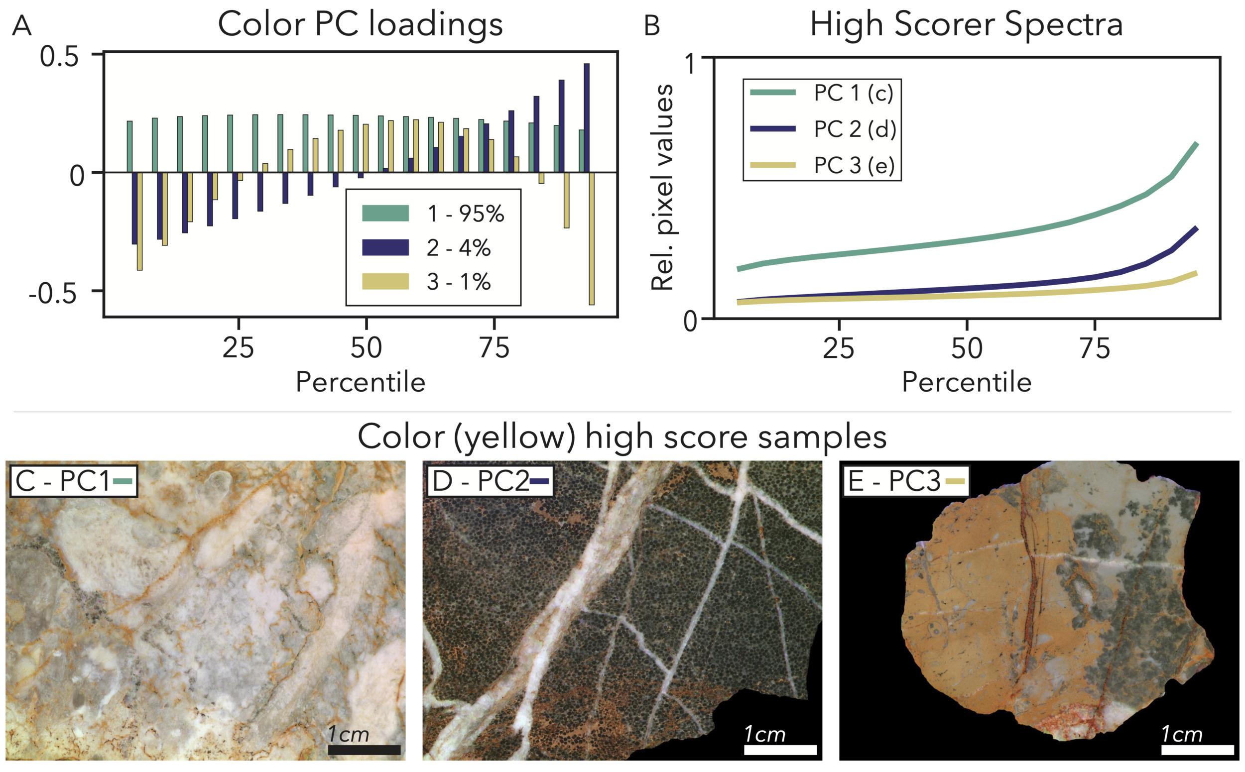
PC1 – Brightness ∼95% variance explained: In each of the color PCAs, the first component explains a large majority of the variance in the data (94– 96%) and generally loads evenly and positively across all percentiles (fig. 8A). This loading indicates that the first PC relates to overall brightness, as is typical for PCAs of color data. High scoring samples in this PC therefore will contain features that are bright regardless of color, like crystalline calcite, as well as features that match the color of that channel. For example, the prevalence of yellow dolomites leads to higher brightness scores in the PCA for the 590 nm (yellow) channel (fig. 8B, C).

PC2 – Light-dark contrast ∼4% variance explained: PC2 explains much less variance (4–5%) across each wavelength and loads very negatively for the lowest percentiles, increasing monotonically to load very positively in the highest percentiles (fig. 8A). This pattern indicates that this PC relates to overall light-dark contrast where the highest scorers will have an even split between very dark features that keep the lowest percentile values low, and bright features that elevate high percentile values, accompanied by a steep gradient between the disparate pixel populations. A high-scoring sample for this PC might have dark shells and ooids, mixed in with bright cements, micrites, dolomites, and calcite veins (fig. 8B, D). While we label this PC as contrast, it is not related to our GLCM contrast metric as this PC does not contain pixel-wise transition information and more refers to the overall color content of a sample.

PC3 – No dark or bright extremes ∼1% variance explained: Much of the remaining variance (∼1%) is explained by PC3, which loads negatively in both low and high percentiles and positively for intermediate percentiles. This PC relates to samples lacking extremely dark or light patches and mostly consisting of intermediate-intensity features (fig. 8B). A good example for a high-scoring rock in this PC again comes from the 590 nm PCA, where the highest PC3 score comes from a sample with a somewhat dark microbial patch, a pocket of medium-gray micrite, and prevalent dolomite (fig. 8E). All of these features moderately-reflect 590 nm light, and the sample does not contain many extremely bright or dark features, like recrystallized calcite.

Figure 8.Dimension reduction of color percentile spectra, showing the 590 nm (yellow) result as an example. Percentile axes in (A) and (B) are the same as figure 7B. (A) A bar plot of loadings gives intuition for the main drivers of variance and interpretation of PC scores from the color spectra, see main text for specific discussion. (B) The percentile spectra of the highest-scoring samples match the overall trends and expectations from the loadings. As examples, the sample from (C) that scores highest in PC1 has high 590 nm reflectance overall, both from bright white sparry calcites and yellow dolomites. The sample in (D) mostly contains dark ooids and so has low values for the earlier percentiles but has prevalent bright calcite veins that cause a sharp increase in the higher percentiles. (e) To score highly in PC3, this sample does not have prevalent elements that are especially bright or dark and mostly comprises gray and yellow colors that give overall-moderate reflectivity.

3.1.2. Texture – GLCM contrast

Prior to performing the PCA on anisotropy size spectra, we normalize these data such that, for each scale, the distribution of values across our sample set has a mean of zero and a standard deviation of 1. We do this normalization step so that the resulting PCs of maximal variance do not disproportionately emphasize size scales with higher magnitudes or variance in anisotropy.

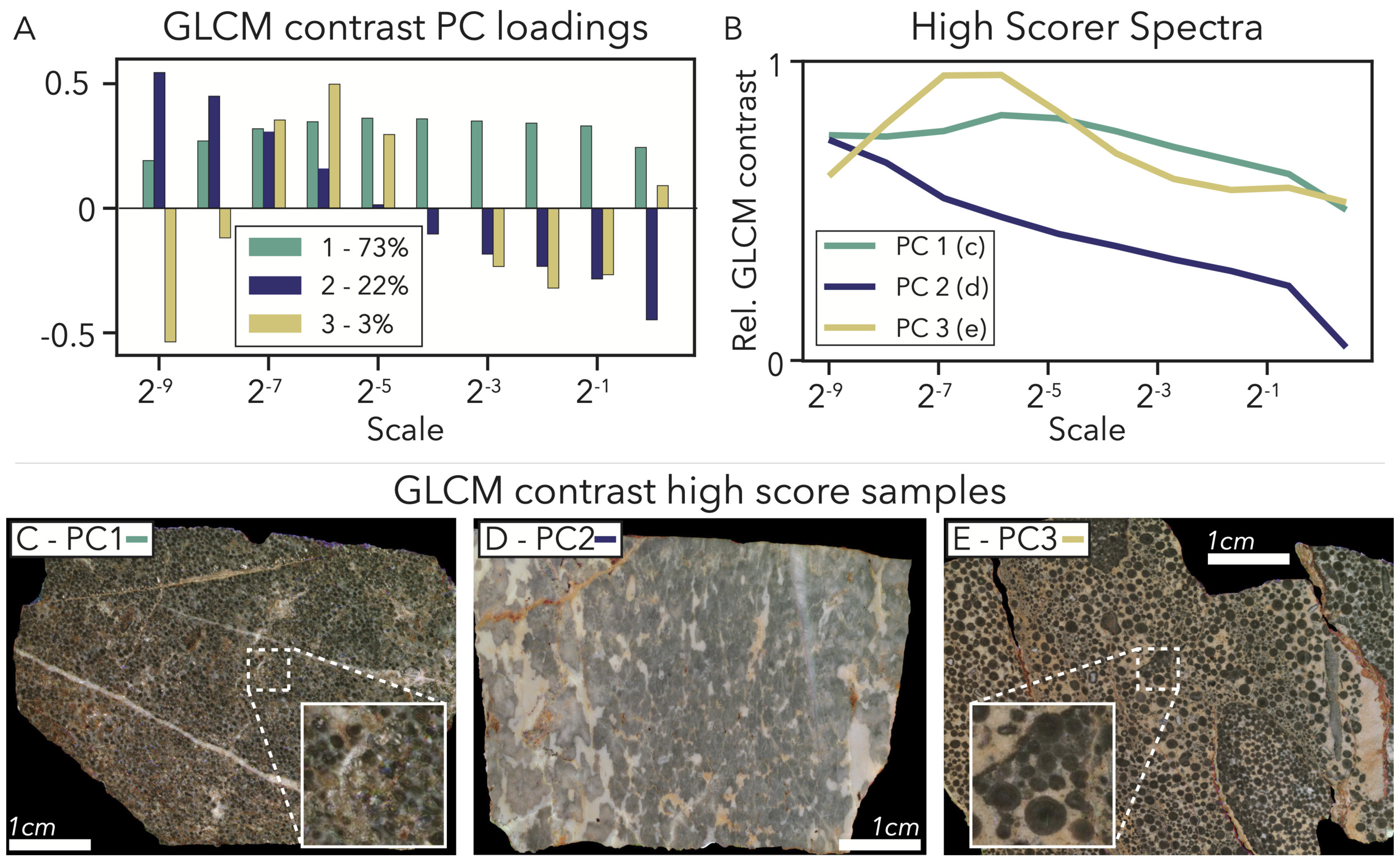
PC1 – Overall GLCM contrast – 73% variance explained: In a similar fashion to the color data dimension reduction, the first component for our GLCM contrast size spectra loads positively across all scales (fig. 9A), implying this PC mainly highlights the difference between high and low contrast samples. The highest scorer for PC1 has a spectrum with high values across the full-scale range (fig. 9B) and strong sources of contrast at all scales. This sample is a fine oolitic grainstone with transitions between dark ooids and cements that give high contrast to the full-scale image, and several large calcite veins and patches that contrast the mostly-dark colors of the sample as the scale shrinks (fig. 9C).

PC2 – Coarse feature GLCM contrast – 22% variance explained: PC2 highlights samples that do not have fine sources of contrast that show up in the full-scale image, but do have contrasting coarser features that are emphasized when the scale shrinks (fig. 9A). This particular scale of contrast could arise from centimeter-scale interbedding of carbonate and siliciclastic material, or in the case of the highest scorer, the presence of coarse microbial patches in a micritic framework (fig. 9D).

PC3 – Contrast from coarse grains – 3% variance explained: PC3 loads negatively for extremely small and moderate-to-large image scales and only loads very positively for moderately-small scales around 2⁻⁶ (fig. 9A). This exact loading is mirrored by the spectrum of the highest scorer (fig. 9B) and reflects contrast at a particular size fraction of grains. 2⁻⁶ is the scale where very fine sources of contrast disappear, but medium-coarse ooids and grains are visible, possibly on much lighter backgrounds like dolomite and micrite (fig. 9E).

Figure 9.Dimension reduction of GLCM contrast size spectra. Scale axes in (A) and (B) are the same as figure 7A. (A) A bar plot of loadings gives intuition for the main drivers of variance and interpretation of PC scores from the contrast spectra, see main text for specific discussion. (B) The contrast spectra of the highest-scoring samples match the overall trends and expectations from (A), and mirror the shapes of the loading curves. (C, D, E) Example images of the highest-scoring samples for each PC highlight the types of features that give contrast at the relevant scales. See main text for specific discussion.

3.1.3. Anisotropy

These data are normalized prior to PCA in the same manner as the GLCM contrast size spectra.

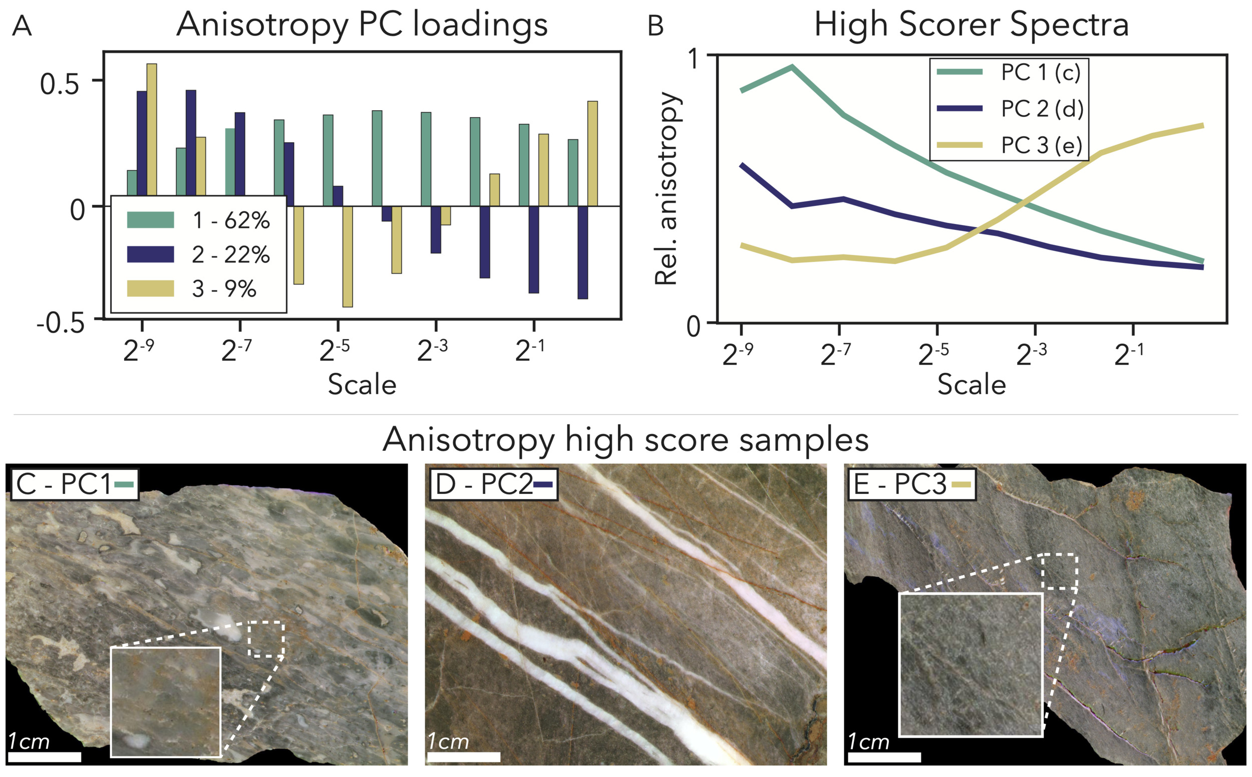
PC1 – Overall anisotropy – 62% variance explained: As with all PCAs thus far, the first PC of the anisotropy size spectra explains a majority of the variance and positively loads at all scales (fig. 10A). This loading indicates that PC1 distinguishes between samples based upon relative levels of overall anisotropy at any scale. The highest-scoring sample for this PC matches that intuition, as its spectrum has mostly-high values (except at the largest image scales; fig. 10B) and its image shows aligned features from fine cracks and veins to coarse micrite and microbial interbeds (fig. 10C).

PC2 – Coarse feature anisotropy – 22% variance explained: PC2 specifically emphasizes anisotropic features that are relatively coarse, and therefore appear disproportionately in the smallest image scales (fig. 10A). The highest-scoring sample from PC1 also has the highest PC2 score, and so to give another example, we show the second-highest scorer, which has thick, well-aligned calcite veins cross-cutting an isotropic microbialite (fig. 10D). When this image is full scale, our anisotropy metric does not rate it exceptionally high (fig. 10B), as fine, nonlinear features like the isotropic microbial texture and crystal faces in the calcite veins give an image gradient that points in all directions. However, when the image is downsampled to the smallest scale, only calcite veins on a homogenous dark background are visible, and the spectrum takes its maximum value (fig. 10B).

PC3 – Fine and coarse feature anisotropy – 9% variance explained: The loading of the third anisotropy PC highlights an even combination of aligned features that are apparent in small and large images, along with the absence of anisotropy in the medium scales (fig. 10A). In the highest-scoring sample for PC3, anisotropy in the full-scale image comes from a fine cleavage fabric, and in the smallest-scale images, its light-dark bedding pattern becomes prominent (fig. 10E).

In our sample set, many features can provide anisotropy, from fine scale veins and cleavage to centimeter-scale bedding. Although our coarse anisotropy metric only capitalizes on the relative distribution of gradient angles in these images, because we assign this metric over a size scale spectrum, we are able to highlight the relative abundance of all aligned features in our sample set.

Figure 10.Dimension reduction of anisotropy size spectra. Scale axes in (A) and (B) are the same as figure 7A. (A) A bar plot of loadings gives intuition for the main drivers of variance and interpretation of PC scores from the size spectra, see main text for specific discussion. (B) As with contrast, the anisotropy spectra of the highest-scoring samples match the overall trends and expectations from (A), and mirror the shapes of the loading curves. (C,D,E) Example images of the highest-scoring samples for each PC highlight the types of features that give anisotropy at the relevant scales. See main text for specific discussion.

3.1.4. Phase modalities

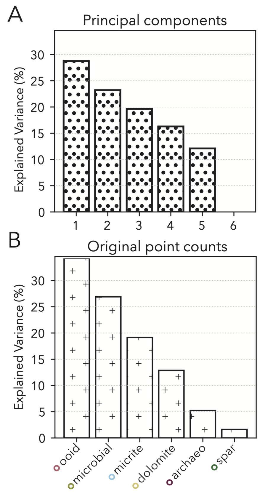
Because we include only the most abundant of our point count classes, our raw dataset of phase modalities only has six metrics (classes). A PCA of these data does not result in components that significantly reduce dimensionality while still including the vast majority of variance. Specifically, we would have to include the first five PCs to explain over 90% of the variance, and no single component is especially useful in capturing a disproportionate amount (fig. 11A). Our raw point count classes have a similar explained variance distribution to the PCs (fig. 11B), and so we elect to keep these data in our final facies vector as individual classes that are more intuitive than PC linear combinations.

Figure 11.Explained variance bar plots for all PCs of point count modalities indicate dimension reduction is not necessary for these data. (A) The explained variance for PCs shows a smooth decline and only significantly drops for PC6, and so we would need to keep the first five PCs to explain over 90% of the variance. (B) The original point count data show a similar distribution of variance explained compared to the PCs. Because these raw data are more intuitive and only require one extra dimension to capture a similar amount of variance, we elect to include these point counts in our facies vector as is.

3.1.5. Geochemistry

Fluctuations in 𝛿¹³C values are primary signals that we are looking to explain with our facies vector, and so we hold that variable out of our dimension reduction and perform PCA just with 𝛿¹⁸O values, Mg, Mn, Fe, and Sr (with the element concentrations normalized to Ca). Following normalization of the dataset such that the relative magnitude of each measurement does not artificially impact loading, we find two significant, intuitive PCs that appear to represent post-depositional diagenetic processes.

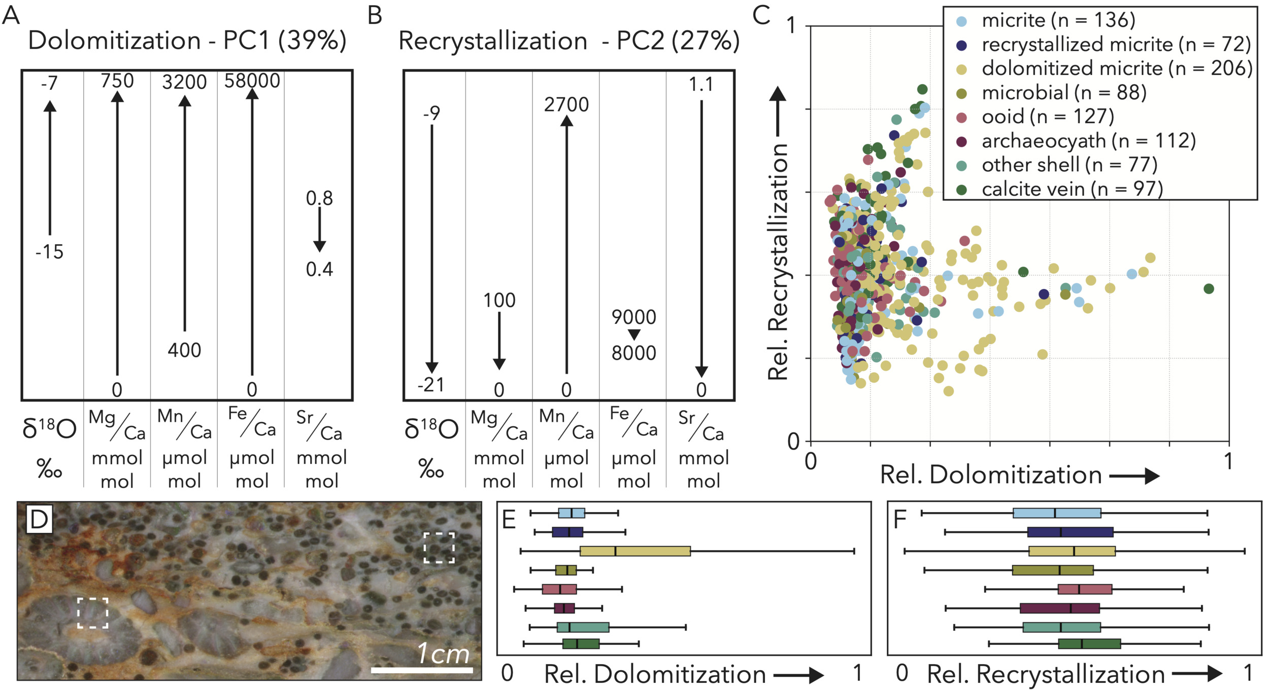
PC1 – Dolomitization – 39% variance explained: The process represented by PC1 likely represents dolomitization. Moving to higher values along PC1 is accompanied by strong increases in Mg, Mn, and Fe content, a moderate rise in 𝛿¹⁸O values, and a small decrease in Sr (fig. 12A). Previous studies have found the chemical signature of dolomitization to include increases in elements like Mg and Fe, along with decreases in Sr as the most pervasive features (Ahm et al., 2018; Husson et al., 2015; Kretz, 1982), which matches our PC1 pathway.

PC2 – Recrystallization – 27% variance explained: This principal component solely is based upon geochemical data. Therefore, the term we use here as recrystallization refers simply to the amount of observed geochemical change in a sample during the process of recrystallization and not any visible textural effects. As samples move higher along the PC2 axis, they sharply decrease in 𝛿¹⁸O values and Sr, see small or no decreases in Mg and Fe concentrations, and a sharp rise in the concentration of Mn (fig. 12B). These signatures, especially the extreme gain of Mn accompanied by loss of Sr, matches previously described chemical changes seen in carbonates in early diagenesis as they recrystallize (Derry, 2010; Jacobsen & Kaufman, 1999; Machel, 1997).

Because recrystallization is pervasive, does not preferentially impact any phases in particular, and can show high scores in samples with well-retained fabrics (fig. 12D), we cannot recognize this alteration process petrographically in our sample set. Thus, we cannot confirm the order in which the two diagenetic processes took place through investigations of cross-cutting relationships. A cross-plot of the two processes does, however, clarify their relative co-occurrences. Specifically, we find that dolomitization is a heavy tailed process that does not severely affect many samples, and the main cluster of points that are most dolomitized only show low-to-moderate recrystallization scores (fig. 12C). Further, the most heavily-recrystallized samples show minimal dolomitization (fig. 12C). Both heavy dolomitization and recrystallization, therefore, likely result in the establishment of a more stable phase that is less susceptible to further alteration by the other process.

Figure 12.Dimension reduction of geochemical data, with 𝛿¹³C values withheld. (A) Arrows show the change in each individual measurement, progressing from the minimum to maximum score in PC1. The length of these arrows relative to the height of the box indicates how much range in a measurement is expressed by PC1 compared to the range of the whole dataset. Numbers at the base of an arrow give the measurement value for the minimum score in PC1, and numbers at the tip give the value at the maximum score. The chemical changes represented by these arrows, like rises in Mg, Mn, and Fe that match the expectation for dolomitization. (B) In the same plot style as (A), we see chemical changes, especially the sharp rise in Mn and fall in Sr, that reflect the expected chemical changes for early recrystallization diagenesis. (C) Cross-plotting all scores for PCs 1 and 2 shows the relative co-occurrences of the two diagenetic processes. For example, the most severe dolomitization tends to occur in low-to-moderately recrystallized samples. Highly-recrystallized samples only show low dolomitization, possibly because recrystallization results in a more stable phase that is less susceptible to further alterations. (D) A portion of an archaeocyath, and a cluster of ooids, both with well-retained fabrics both scored above the 88th percentile of recrystallization score. This example shows that recrystallization does not have any pervasive textural or fabric-destructive indicators, and instead refers to the amount of geochemical change imparted during recrystallization. Colors in (E) and (F) are after the legend in (C). (E) Phase-wise distributions of geochemical PC1 illustrate a phase-wise trend in that dolomitized muds preferentially are more impacted by dolomitization. (F) Recrystallization has no trend in terms of a particular class being more or less affected.

3.2. Overview of the facies vector

Following all PCAs, we now have a vector reduced to 36 metrics that represents lithologic components, such as phase modality, relative feature sizes and alignment derived from image analyses, and geochemical alteration processes (fig. 13A, B). We also add the stratigraphic height of each sample as its dip-corrected elevation, providing a variable that represents an estimate of chronologic order to check temporal trends in samples. Although cryptic cut and fill structures can add uncertainty to relative chronologies from stratigraphic position (Geyman et al., 2021), this metric is our best approximate indicator. With this vector, we can return to our research questions asking: do depositional environment and/or diagenesis contribute a high degree of variability relative to outcrop signals, and explain patterns in 𝛿¹³C values and fossil occurrences? After we have understood those patterns, does our study outcrop retain any residual signs of secular change over time?

To direct our search in understanding trends in 𝛿¹³C values and fossil occurrences, we start by looking for correlations between these variables and our facies vector components. For 𝛿¹³C values, we look at the Pearson coefficient. Because fossil occurrences are binary, we look at how much more explanatory power a logistic regression of a given metric against occurrences has over random 50–50 chance. In this exploratory exercise, we note several relationships to investigate further.

𝛿¹³C values have strong negative correlations with our geochemical PC2 that represents recrystallization, along with stratigraphic height (fig. 13C). For lithologic variables, we see moderate, negative correlations between stable carbon isotope ratios and contrast PCs 1 and 3, pointing to a possibility that heterogenous grains and coarse ooids could be prevalent in samples with low 𝛿¹³C values. Anisotropy PC3 also negatively correlates with carbon isotope ratios, so either bedding or fine-scale cleavage cracking merit further investigation in driving lower values. The slight positive correlation between microbial fraction and 𝛿¹³C values indicates that the presence of microbially-bound substrates could be promoting higher ¹³C/¹²C ratios.

Predictability of fossil occurrences given our facies vector gives many potential variables to investigate further. A metric that perfectly predicts any fossil group would have a logistic regression improvement of 1. Thus, the maximum improvement we see of ± 0.3 (fig. 13C) demonstrates that no individual variable is a strong predictor of fossil occurrences. However, the abundance of metrics that do give some improvement (fig. 13C) support the idea that our facies vector captures properties that have a relationship with fossils, and motivates a more complex analysis that attempts to explain occurrences through a combination of variables.

Figure 13.Overview of results after compiling a dimension-reduced facies vector and regressing with significant variables. (A) We visualize the results of our method by taking each sample on our map and replacing it with a quantitative barcode, like (B), where the brightness of each strip refers to the sample’s relative color, contrast, recrystallization, etc. (C) With these barcodes, we can start to look for patterns. Aside from assessing trends within facies vector components, we regress all variables against the 𝛿¹³C values and fossil occurrence data we want to understand in light of depositional environment and diagenesis. We find several possible significant correlations to investigate further, like between geochemistry PC2 (recrystallization) and 𝛿¹³C values, along with contrast PC2 with most fossil groups.

3.3. Diagenetic contribution to 𝛿¹³C values

Because the negative correlation between 𝛿¹³C values and the degree of chemical alteration during recrystallization (geochemical PC2) is strong, a closer investigation of that relationship is a clear first step in gathering a more mechanistic understanding of diagenesis within this outcrop. We saw in our outline of the geochemical PCs and figure 12D, E that recrystallization’s chemical effects are not indicated by a particular petrographic fabric, nor are they preferentially associated with any phase. This diagenetic process also impacts micrite samples, which is the most often-used phase when determining secular trends on carbonate platforms (Bergmann et al., 2018; Goldberg et al., 2021; Kaufman & Knoll, 1995; Knoll & Walter, 1992; Saltzman & Thomas, 2012). Therefore, although previous studies have had success avoiding certain diagenetic processes through petrographic identification of samples with excellent fabric retention (Bergmann et al., 2011; Hood et al., 2016), recrystallization is not a factor we can ignore at this outcrop through similar sub-selection (fig. 12D).

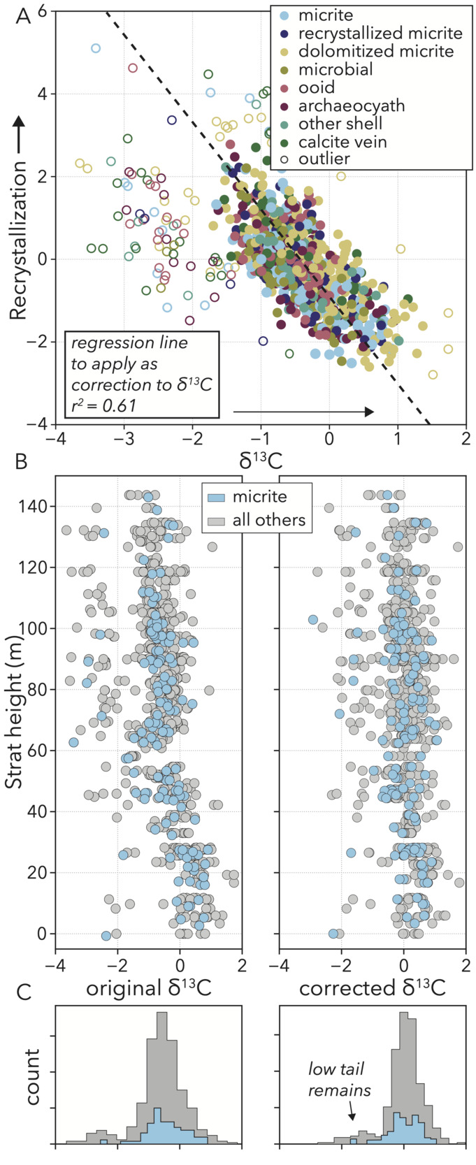
The relationship between 𝛿¹³C values and recrystallization is approximately linear, save some samples that fall off the main trend towards lower 𝛿¹³C values (fig. 14A). To better understand how this process is expressed in our samples, we use the equation of the regression line that fits the main cluster as a correction factor. Based upon how far each sample is along the recrystallization axis, we add the corresponding 𝛿¹³C value to remove the negative trend.

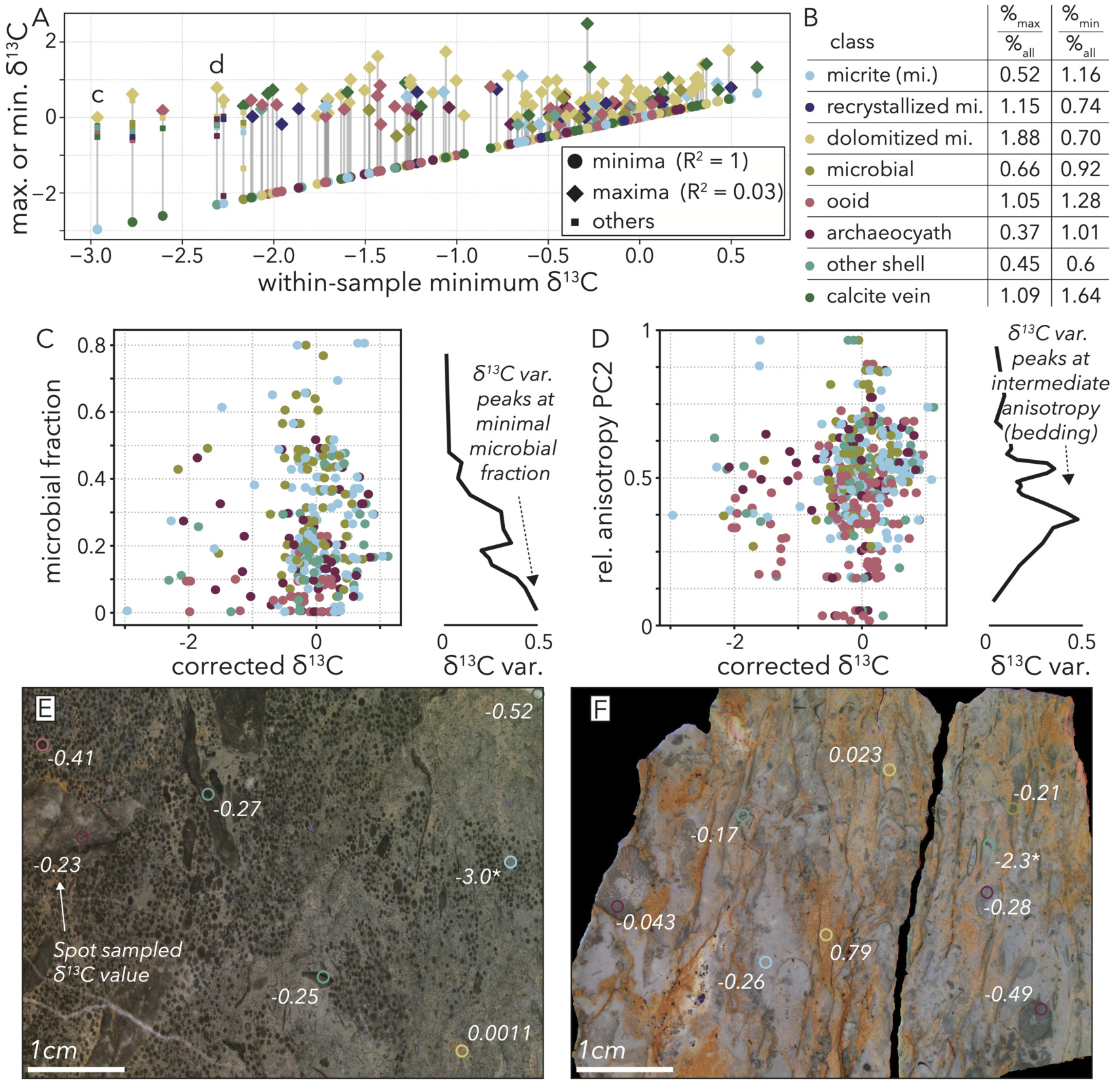
Prior to correction, the record of stable carbon isotope ratios when looking at all samples in stratigraphic position shows an overall ∼2‰ decline over the course of the section (fig. 14B), which is why 𝛿¹³C values and stratigraphic height have a strong negative correlation (fig. 13C). In addition to this general trend, the curve shows high variance along strike, with a fairly-constant range of ∼4–5‰ throughout. 92% of samples are closely clustered in a ∼2‰ range along strike with variance stemming largely from a group of samples that form a separate, more negative cluster (fig. 14C). With both along strike variance, and the general stratigraphic excursion being negative trends, either could be related to recrystallization.

Following correction, the main population of samples now centers around 0‰ with no trend over the stratigraphy (fig. 14B), but the separate population with more negative values remains (fig. 14C). Therefore, the negative correlation between 𝛿¹³C values and recrystallization represents a stratigraphic trend in alteration where higher-up samples are more impacted. Accounting for recrystallization removes any apparent secular trend in 𝛿¹³C values, strengthening the conclusion of isotopic stasis reached by previous authors (Rowland et al., 2008). However, the remaining ∼4–5‰ range along strike, even among micritic samples, requires explanation. Is some other diagenetic imprint driving certain samples to more negative values, or is this range representative of contemporaneous variation in carbonate bulk sample 𝛿¹³C values like we see on the GBB today?

Figure 14.A recrystallization explanation for the stratigraphic trend towards lower 𝛿¹³C values. (A) A cross-plot of our recrystallization PC and 𝛿¹³C values shows no clear trends in terms of particular phases clustering around certain geochemical values. The main cluster of non-outlier points (determined through visual inspection) does have a strong, linear, negative correlation, which can be applied as a correction to remove the influence of recrystallization from 𝛿¹³C values. (B) When plotted versus stratigraphic height, the original 𝛿¹³C values show a general ∼2‰ decrease, and a ∼4–5‰ range along strike. These trends apply when isolating just micrite samples, as well as looking at the entire dataset. Following correction for recrystallization, the negative trend over stratigraphy is removed, but the range along strike remains. (C) Histograms of 𝛿¹³C values before and after correction show the bimodal nature of carbon isotope ratios, with a small population of samples with low 𝛿¹³C values that remain even after correction.

3.4. Lithofacies contribution to 𝛿¹³C values

The geochemical portion of our facies vector does not hint at any other diagenetic factor that could produce the population of samples with low 𝛿¹³C values. Although we do not correct for dolomitization (geochemical PC1), that process only positively correlates with 𝛿¹³C values (fig. 13C) and mostly drives maximal values in the dolomitized micrite class (figs 12C, 15A, B). Further, because the lowest stable carbon isotope values are not disproportionately associated with dolomitized micrite (fig. 15A, B), dolomitization is unlikely to be driving this variance.

Several lines of evidence point to at least a portion of the population with low 𝛿¹³C values as sampling original variance that was present at burial. Our sampling technique involves drilling 4–12 separate areas per polished slab, and variation in 𝛿¹³C values within each hand sample do not indicate that certain rock samples were diagenetically overprinted with lower values by processes undetected by our geochemical PCA. When we plot within-sample maxima versus their corresponding minima, we do not see any positive correlation that would be expected if low 𝛿¹³C values were preferentially coming from hand samples that are isotopically light overall (fig. 15A).

Some of the variability in lower 𝛿¹³C values does stem from the presence of calcite veins, as sample minima are disproportionately assigned to this class (fig. 15B). However, hand samples that do have a very low 𝛿¹³C value associated with a calcite vein do not show other sample points being driven to negative values along with the vein (fig. 15A). While veins can vary between very high or low 𝛿¹³C values (fig. 15A), there is no evidence that the prevalence of this phase overprints even the most nearby sample points (fig. 15A, C). Of the 53 sample minima that are lower than -0.8‰, the approximate break point in the bimodal distribution of corrected 𝛿¹³C values (fig. 14C), only 11 are from the calcite vein phase. Therefore, 42 samples have low minimum stable carbon isotope values that cannot be explained through geochemically-detected diagenesis or petrographically-visible fabrics.

Because individual rock samples themselves have variable 𝛿¹³C values depending on which phase was drilled (ranges of > 3‰ are common), we seek to understand what drives within sample variance to low values. Comparing our lithofacies metrics to observed variance in 𝛿¹³C values, we find two variables with potential explanatory trends. Specifically, we find a peak in variability of 𝛿¹³C values (driven by low values) associated with minimal microbial content (fig. 15C), as well as intermediate anisotropy PC2 values most associated with bedding (fig. 15D). These trends, derived from image analyses, introduce the idea that variability, and specifically the inclusion of lower values, in 𝛿¹³C value primarily relates to the concentration of disparate, allochthonous materials in bedded deposits. Microbialite is not expected to be a primary component in ex situ deposits, save rare rip-up clasts, and bedding is a clear sign of secondary deposition. Therefore, just as the most chemically variable facies on the GBB today are those that juxtapose in situ corals or foraminifera with allochthonous mud (Geyman & Maloof, 2021), we find that deposits consisting of disparate, washed-in grain types can have within-sample variability greater than any observed stratigraphic trend in this Cambrian outcrop. Qualitative petrographic observations, while not the basis of our analysis, also support what we find in the quantitative trends. Observing the sampled areas with the lowest 𝛿¹³C values, we see examples such as a micrite pocket in an otherwise coarse ooid and shell debris packstone (fig. 14E), and a shell fragment in a coarse, proximal reef debris deposit (fig. 15F).

Figure 15.A lithofacies explanation for phases with low 𝛿¹³C values. (A) To visualize the distribution of 𝛿¹³C values from all phases drilled from a single sample, we plot the within sample maxima and minima versus the minima. There is no trend between maxima and minima, and when we plot the intermediate points for the six leftmost samples, we see that most points remain closely associated with the maxima (we only show these few just to illustrate the point without overcrowding the plot). Because the maxima are most often dolomites, it is possible that dolomitization is a homogenizing factor (Ahm et al., 2018) pulling values overall towards ∼+0.5‰. (B) To see if a certain phase disproportionately accounts for maxima and minima, we calculate the ratios between the percentage of times a phase constitutes either the max. or min. versus the percentage that phase constitutes in all geochemical samples. A value of 1 for this ratio would indicate the phase is the max. or min. a proportional number of times given its membership in the overall dataset. From these ratios, we see that dolomitized micrites disproportionately account for maxima, in line with the conclusion from figures 12F & 13C, and that dolomitization is associated with relatively high 𝛿¹³C values, specifically where petrographically visible. Calcite veins also disproportionately account for minima, indicating this class is more prone to lower isotope values, but we do not see any evidence of veins impacting 𝛿¹³C values in nearby drill points in the same hand sample in (A). (C,D) In plots containing only non-diagenetic classes (excluding calcite veins, recrystallized and dolomitized micrite), facies vector components show relationships with 𝛿¹³C values that align with the interpretation that variability in 𝛿¹³C values relates to bedded, allochthonous deposits. See main text for further discussion. (E) The hand sample that contains the lowest minimum value in our dataset is an oolitic and skeletal debris packstone with well-retained fabrics. The sampled spot that yielded the minimum (marked with an asterisk), is a micrite pocket that does not show geochemical or petrographic signs of alteration. (F) The hand sample that contains the fourth lowest minimum value is a coarse packstone with proximal reef debris. Although this sample shows prevalent dolomitization, that phase only is associated with higher 𝛿¹³C values, so the minimum value from one of the sampled shells likely does not stem from that diagenetic process.

3.5. Influence of lithofacies on fossil occurrences

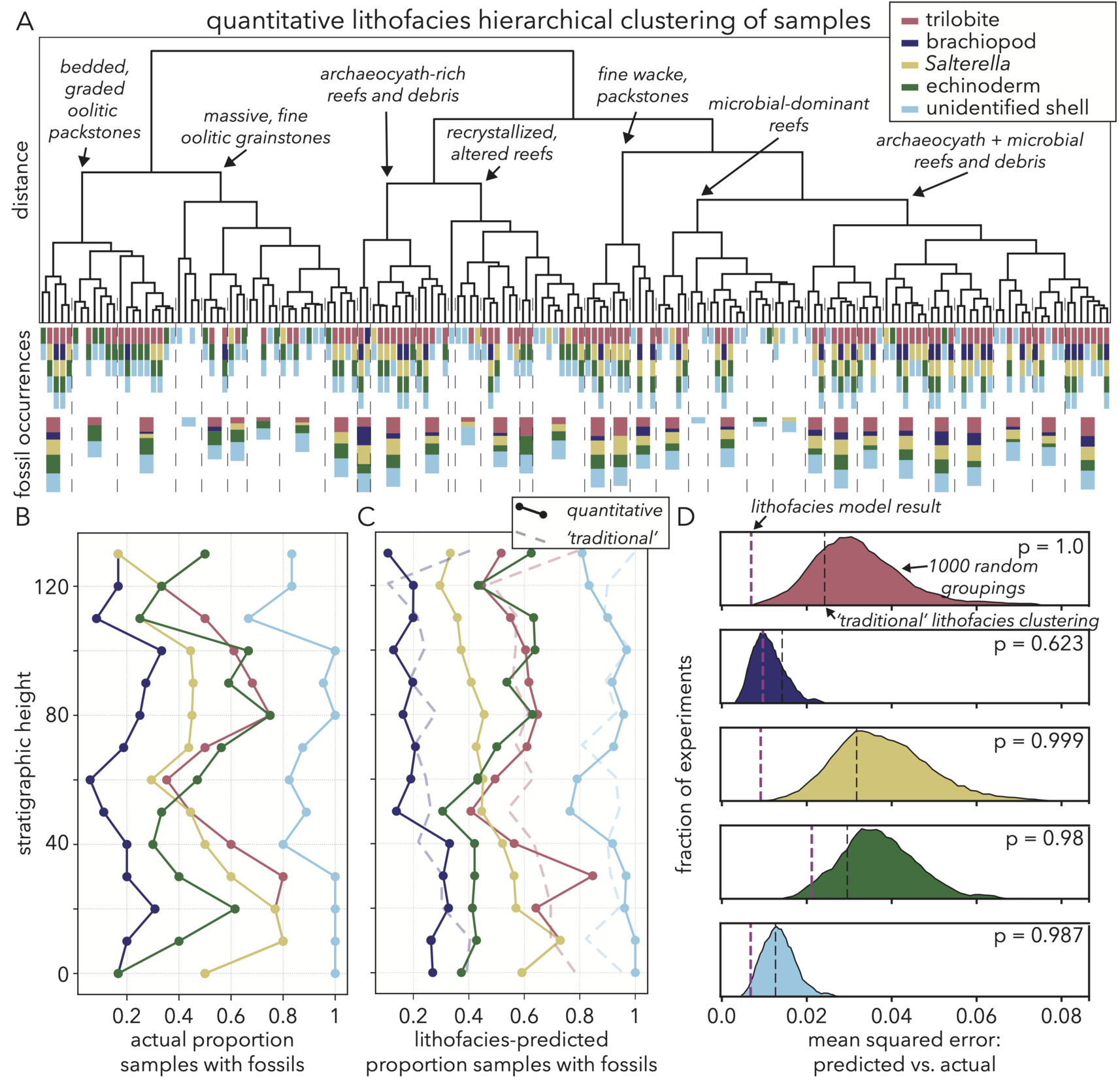
Fossil occurrences are the other critical variable to explain in our Cambrian section as we look to understand trends in biodiversity and the potential influence of depositional environment. Specific to our study motivations, we want to know if any or all fossil groups show strong associations with particular lithofacies that may dictate interpretation of stratigraphic trends and pinpoint if reef environments are a driver of fossil occurrences. We start this exploration by using the lithological metrics in our facies vector to perform a distance-wise hierarchical clustering of all samples (fig. 16A; Bonham-Carter, 1965; Parks, 1966), an analysis only possible with our quantitative image metrics. Because our goal is to understand lithofacies influence on fossil occurrences, we sub-select a set of metrics for this hierarchical clustering that have relatively large logistic regression improvements (fig. 13C) with at least one fossil group. The list of metrics we cluster on is GLCM contrast PC2,3, anisotropy PC2,3, microbial fraction, dolomite fraction, ooid fraction, archaeocyath fraction, UV (365 nm) PC1, and yellow (590 nm) PC1.

Like the dimension reduction explanations for lithofacies metrics, this clustering result helps confirm that the facies vector captures relevant sample features, as the hierarchy gives intuitive groupings. For instance, the various types of oolites are perhaps the most distinctive samples to a geologist in terms of grain modalities, color, and texture, and these rocks form their own cluster separate from reefs and other bedded deposits (fig. 16A).

More importantly than reproducing categories that make sense to a geologist, this quantitative clustering offers the opportunity to further subdivide the main six lithofacies seen in the field (fig. 3), with consequences for interpreting the partitioning of fossils. As an example, our field survey, along with previous studies of this section (Rowland, 1984; Rowland & Gangloff, 1988) note a distinction between lower and upper reefs accompanied by a possible increase in archaeocyath abundance. The lithofacies clustering then goes a step further and subdivides a category like the microbial-dominant reefs typical of the lower parts of the section. These samples are organized based upon slight differences in bedding textures or the inclusion of other carbonate constituents that indicate changes in depositional environment in the same overarching lithofacies category (fig. 16A). This subdivision of lithofacies is crucial for interpreting fossil occurrences, as within a category like microbial reefs, some subgroups have abundant, diverse fossils, while others remain sparse (fig. 16A).

The implications of this fine-scale quantitative lithofacies subdivision for interpreting biodiversity signals can be shown stratigraphically. Without knowledge of lithofacies, fossil occurrences binned into 10 m stratigraphic windows show several trends to investigate. Salterella is the only group that shows a significant decline throughout the section, and resembles all other groups in having a local minimum in occurrences from 40–60 m (fig. 16B). These local minima are surrounded by ∼30 m intervals of relatively high prevalence where all groups, save brachiopods, are present in over half of the samples (fig. 16B).

We test the importance of relative depositional environment in creating these trends by using the clustered lithofacies groups and their fossil abundances to produce stratigraphic trends expected given lithological variability⁠ (fig. 16C). Specifically, in each stratigraphic window, we multiply the fractional membership of lithofacies groups by the proportion of samples within each group that have a given fossil. The result is a model that forms the null expectation for fossil occurrences that are entirely predictable given quantitative lithofacies. For comparison, we create a similar predictive model based upon ‘traditional’ carbonate petrological data available for our samples, such as Dunham classification (Dunham, 1962) and point counts. To test the significance of both the quantitative and traditional lithofacies model explanations of fossil occurrences, we also perform an experiment randomly clustering samples 1000 times into groups of the same size as the lithofacies model. For each random set of groupings, we then calculate the expected proportion of fossils in each stratigraphic window with the same protocols as with the lithofacies model.

The quantitative lithofacies-predicted fossil occurrence model matches the vast majority of trends in actual fossil occurrences, both in timing and magnitude (fig. 16B, C). As examples, this model reproduces the decline in Salterella proportions from 0.7 to 0.3 over the entire section, along with the decline and subsequent rise in trilobites between 30 and 70 m, and the rise in echinoderms from 0.3 to 0.6 between 50 and 80 m. The only fossil group that is not well explained by lithofacies is brachiopods, which rise from near 0 to 0.4 in actual occurrence proportions between 60 and 100 m. This trend is not seen in the lithofacies model and may represent a real, yet small rise in brachiopod abundance, or a shortcoming in our lithofacies quantities in capturing the dependence of brachiopods on depositional environment. For all fossil groups except brachiopods, the quantitative lithofacies model is significantly more accurate than random groupings in reproducing the actual stratigraphic fossil trends (fig. 16D). The quantitative lithofacies cluster model also consistently outperforms the model based upon traditionally-available data (fig. 16D). Therefore, we are able to explain all significant trends in fossil occurrences through relative proportion of lithofacies, and that result only is likely to happen when samples are grouped in a directed manner guided by quantitative lithofacies characteristics that capture paleoenvironment and taphonomy.

We find that lithofacies adequately explains nearly all patterning in fossil occurrences. Specifically, almost no fossil groups appear in microbial reefs (fig. 16A), and because that lithofacies occurs most prevalently at the base of the section and between 40–60 m, that minimal fossil association gives rise to the first two minima in occurrences (fig. 16C). Salterella, which shows a consistent decline in occurrences, is not strongly associated with oolites, but occurs in nearly all non-microbial reef lithofacies. Salterella is unlikely to be found in oolites, as its shell is fine and small, liable to be broken easily in transport, and in most cross-sections resembles an ooid. Thus, even in examples near oolites, this fossil is restricted to the reefs. Echinoderms are nearly the opposite as their plates are robust and easily recognizable in most cross-sections, and so while they are prevalent in reefs, they also often can be found in associated debris beds. Their occurrences simply rely on the reefs not being strictly microbial. In the case of all fossils, we find their occurrences to be highly patterned by lithofacies, where animals lived in and around reefs built by archaeocyaths. This discovery indicates that when we change our study approach to capture lateral variability and small-scale sub-environments, we may be more likely to recognize influences on biodiversity, such as reefs (fig. 2), that are difficult to measure with traditional stratigraphic techniques.

Lithofacies associations of Cambrian fauna have been noted by previous authors. For example, Jacquet et al. (2019) find that small shelly fossils of the Arrowie Basin, South Australia have a high correlation with depositional environment, noting that the lithofacies associations most closely track where each faunal group is expected to be preserved. While we cannot rule out that the lithofacies associations we find in this study are driven by diagenesis and preservation, we find it unlikely that these two factors drive the trends. The stratigraphic curves of most fossil groups peaking both near 30 m and 90 m (fig. 16C) do not match the monotonic trend of chemical diagenesis in the form of non-fabric-destructive recrystallization (fig. 14B), and so we have no evidence of preferential shell dissolution in certain samples. Further, the environments in which we most often find fossils are archaeocyath-rich reefs and their associated debris (fig. 16A). Due to the coarse and porous nature of reef sediments, these environments are perhaps the least likely to preserve recognizable associated taxa (Hubbard et al., 1990, 2001; Wood, 1999). Therefore, the fact that reef lithofacies are a significant predictor of fossil occurrences probably indicates a true ecological affinity of these groups for reef environments (Pruss et al., 2025).

Figure 16.A lithofacies explanation for fossil occurrences. (A) We perform a hierarchical clustering, using Ward’s method (Ward Jr, 1963), on our samples based upon lithological metrics the facies vector and find intuitive groups and relationships. Within these groups, fossil occurrences appear deterministic. For example, many fossil groups are completely absent from oolites and microbial reefs, showing preference for reefs with archaeocyaths or their accompanying debris deposits. (B) To pinpoint the degree to which the quantitative lithological descriptors and their resulting clustering can explain fossil occurrences, we start by visualizing the proportion of samples containing each fossil group in 10 m stratigraphic windows. (C) When we calculate the expected stratigraphic trends in fossils by multiplying the proportion of occurrences in each lithofacies group from (A) by the frequency of each lithofacies group in the stratigraphic windows, we reproduce the major features from the curves in (B). For example, we see a similar rise in echinoderms between 40 and 80 m, a decline and recovery of trilobites in the same interval, and a general decline in Salterella from 0.7 to 0.3 throughout the entirety of the section. We are able to reproduce these signals with a model that does not have stratigraphic information encoded and simply takes in fossil associations with quantitatively-determined lithofacies groups. A separate predictive model, based solely on ‘traditional’ lithofacies data, like Dunham classification (Dunham, 1962) and point counts does not reproduce the real stratigraphic trends as accurately. For example, this traditional model does capture the overall decrease in trilobites with increasing stratigraphic height, but fails to replicate the large 2^nd order decrease from 30–50 m. We only show three of five fossil classes for the traditional model to reduce clutter in the figure.(D) This result is significant, as the stratigraphic relationships in (B) are not likely to be reproduced by chance. We perform an experiment where we create sample groups of the same sizes as in (A), but randomize sample membership over 1000 runs, and in each run we calculate the predicted stratigraphic trends in all fossils, as in (C). For all fossils, save brachiopods, the mean squared error between predicted and actual occurrences is significantly low for the lithofacies model compared to the random draw experiments. In all cases, the model based upon our nuanced, quantitative lithofacies vector significantly outperforms the ‘traditional’ clustering model. The failure of both facies models to accurately predict brachiopod occurrences may stem partly from generally low proportions of occurrences for the group throughout the section, limiting ability to establish robust facies associations.

3.6. Implications for Cambrian environmental change

We are unable to reject the null hypothesis that depositional lithofacies and diagenesis are the primary source of stratigraphic trends in 𝛿¹³C values and fossil occurrences, and find no evidence of broader environmental turnover in this outcrop. In other words, we find very little signal of secular change relative to identified sources of internal variability. Raw data from this locality could be interpreted as showing a ∼2–3‰ negative excursion in 𝛿¹³C values (fig. 14B), accompanied by at least two downturns in fossil abundance (fig. 16A). Measuring a single section instead of taking a grid approach can amplify those conclusions, showing an additional 2–3‰ negative excursion in 𝛿¹³C values that overlaps with a disappearance of most fossil groups. Studying the intersection of lithofacies, diagenesis, and original environments, however, we recognize a platform in steady state where overall 𝛿¹³C values of micritic samples remain constant near 0‰, accompanied by phase-wise variability of greater than 4‰ at the time of deposition, and fossil occurrences largely explained by the style of reef environment available in each stratigraphic interval.

Our result of relative stasis is not devoid of opportunities to learn about Cambrian environments and the nature of the geologic record. Geology and Earth history often are the fields of identifying environmental change over time in order to understand feedbacks between surface processes and the biosphere that impact the co-evolution of life and environment on our planet. The goal of understanding this co-evolution may be to offer constraints on possible future states of the Earth-life system. Our review of current literature on modern environments and results in this study, on the other hand, indicate that lessons from very recent Earth history offer necessary perspective for interpreting the deep past.

The Cenozoic Era, which is of similar duration to the Cambrian period, has several examples of large-scale overturn. In just over 65 million years, Earth went from an ice-free hothouse to having large ice sheets near the poles that can drive ∼100 m sea level fluctuations (Dingle et al., 1998; Hambrey et al., 1991; Zachos et al., 2008), the number of marine families nearly doubled (Sepkoski, 1981), and the entire Tibetan Plateau was built (Harrison et al., 1992). Specifically looking at carbon cycling throughout this interval, the record of 𝛿¹³C values measured from benthic foraminifera—which are expected to faithfully track global ocean DIC—remains within an approximate 2‰ window (Zachos et al., 2008). Each of the events listed above could have large causes or consequences within the carbon cycle, but when we interpret the state of marine DIC through a reservoir that has much less internal variability than a carbonate platform, we do not see a sequence of largescale step changes. Instead, given the benefit of a more complete, recent record, the Cenozoic appears as a time where small, gradual, and perhaps even imperceptible forces can produce grand change.

Of course, the Cambrian and Cenozoic show measured differences in the Earth system, especially with relation to influences on the DIC pool. Some characteristics of the Cambrian, such as a lack of a land biosphere (Algeo et al., 2001; Berner, 1997) and planktonic calcifiers to provide a deep ocean carbonate buffer (Kvale et al., 2021; Ridgwell & Zeebe, 2005), or an underdeveloped biological pump (Meyer et al., 2016; Steinberg et al., 2008), may have enhanced volatility in the DIC pool to create conditions for real, large-scale changes in the carbon cycle. At the same time, the DIC pool was much larger in the Cambrian than the Cenozoic, and may have been more stable than what we observe over the last 65 million years (Bartley & Kah, 2004). The lever can pull both ways, and we are not arguing here for any particular mechanism, or that all of Earth history was shaped by uniformitarian phenomena. However, the fact that the first time we applied nuanced methods to quantify depositional environment on a rock outcrop, nearly all chemical and biodiversity signals could be explained through the environmental variability represented by lithofacies, implies there is more work to be done. Although correlated stratigraphic signals between sections may at first glance suggest sudden, global causes, both the Cenozoic literature, and the results of this study indicate that uniformitarian behavior may be a more common agent of change that can produce dramatic results. Have we truly overestimated global environmental overturn in the Cambrian? Time will tell what we can learn from this important interval, and others, in Earth history as we continue to assess S:V, and disentangle sub-environmental variability from secular stratigraphic signals.

3.7. Future work

A main objective of our study, aside from any particular geological conclusions, is to introduce an approach and a way forward for continued work interrogating signals and constraining the role of lithofacies. A key component of future work will be to expand to more outcrops to place context on the results we achieve herein and ask follow-up questions. For instance, while we recognize a preference among animal fossils for archaeocyathan reef environments compared to other lithofacies available at this outcrop, does that preference still hold when we sample the broader lithofacies mosaic available on the Laurentian paleocontinent of the early Cambrian? While collecting and processing over 150 samples on a single outcrop likely is too dense a sampling to achieve broader coverage in any reasonable timeframe, sample density can be tailored to the question at hand. We choose a 10 m grid spacing to match the apparent lengthscale of reefs at outcrop, but future sampling strategies can be designed to fit outcrops with longer lengthscale transitions or basin-wide questions. Additionally, because all samples are archived with an image and GPS point, no study is done in isolation. If future work needs to pool multiple outcrops, fill in gaps with more serial sampling, or add additional context to samples, such as mapped outlines of reef mounds or regional dolomitization fronts, previous image archives will allow the community to easily build off what has already been done.

This study and the computer vision metrics we apply also only represent a start in the process of supplementing expert domain knowledge with rich archives and reproducible methods. We are hopeful that as high throughput petrographic imaging gains broader adoption, the suite of computer vision tools to assess lithofacies characteristics grows alongside, especially as studies point to aspects that would be helpful to constrain. In this study, for example, we do not find a fabric retention/destruction relationship with diagenesis, but that concept may be better tested with metrics specifically suited to capture petrographic signs of diagenesis, as opposed to depositional environment. In the coming years, AI likely will see increased application as models become more powerful and toolkits improve ease of use. An AI model that automatically segments petrographic images so we can replace the point counts used here with full area or volume fractions would provide for faster, more specific insights. Now is a crucial time to be engaging with image archives to learn as a community what properties we want to quantify through intuitive methods, like those presented herein, and which measurements should be automated through less-interpretable AI applications. The development of AI tools and bespoke methodologies themselves does not in itself represent an advance in geological insights, and so we need to outline which developments will improve our observational power to learn more about the nature of Earth history. While leveraging computer vision and other computational techniques increase the amount of research geologists can do at a distance from rock outcrops, we hope these methods make for closer examination of the geologic record.

Acknowledgments

The authors would like to thank Akshay Mehra, Sarah Ward, and Sarah Brown for help conducting field work. Emily Geyman coined the term ‘facies vector’ and helped conceptualize quantitative lithofacies methods. Julia Wilcots provided insights on the interpretations of geochemical data. Cedric Hagen helped in developing the computer vision methods. We thank Mark Webster for thoughtful discussions and comments on early drafts that helped improve the quality of the research. We sincerely appreciate the valuable comments and suggestions from our reviewers and associate editor, which have significantly improved the quality of this manuscript. Funding for this project came from National Science Foundation grants 1410317 and 1028768 to A.C.M., as well as the Tuttle Invertebrate Fund and the Geoscience Student Research Fund at Princeton University.

Data availability

We have created a repository with Princeton Data Commons (doi: https://doi.org/10.34770/bm0d-q534) that holds sample images, geochemical data, and analysis codes used for this study.

Editor: C. Page Chamberlain, Associate Editor: Amanda M. Oehlert