


1. INTRODUCTION
The chemical weathering of continental crust is thought to regulate Earth’s climate on million-year timescales (Hilton & West, 2020; Urey, 1952; Walker et al., 1981). Acid-base and redox reactions involving crust-forming minerals like silicates, carbonates, and sulfides impact the alkalinity (ALK) and dissolved inorganic carbon (DIC) of water that mediates these reactions. Together, the net change in ocean-atmosphere ALK (∆ALK) and fluid inorganic carbon (∆FIC, equal to the sum of atmospheric CO2 and DIC; Kemeny et al., 2024) generated by these reactions modulate the apportionment of carbon between the ocean and atmosphere, meaning that chemical weathering alters atmospheric carbon dioxide (pCO2) levels over a range of time scales. The principal reactions that impact marine ALK and FIC, assuming a balanced organic carbon cycle, are the weathering of carbonate and silicate minerals by carbonic and sulfuric acid (R. A. Berner et al., 1983; Stallard & Edmond, 1983). However, the formation of secondary phases like carbonates, clay minerals, and oxides following the weathering of primary minerals variably alter the net ALK and FIC fluxes associated with chemical weathering. Understanding how secondary phase formation impacts the net ALK and FIC fluxes due to chemical weathering thus has first-order implications for understanding both planetary habitability over geological timescales and for quantifying the net impact on pCO2 due to enhanced rock weathering interventions.
The balance of all near-surface weathering reactions dictates whether, and over what duration, chemical weathering causes an increase or decrease in pCO2. Carbonic acid weathering underlies the longstanding expression of the silicate weathering feedback (Walker et al., 1981). The first step in this feedback is the weathering of carbonate minerals (eq 1) and silicate minerals (eq 2), followed by production of marine CaCO3 (eq 3). Where the first equation produces ALK, the third equation removes ALK.
CaCO3+2H+→ Ca2++H2CO3
12CaβNa2(1−β)SiO3+H+→β2Ca2++(1−β)Na++12SiO2+12H2O
H2CO3+Ca2+→ 2H++CaCO3
The value of sets the balance of alkali and alkaline metals silicate supply. When =1, the sum of equations (2) and (3) represent the classical “Urey reaction” (Urey, 1952), which simply conveys that for one mole of ALK generated by silicate weathering, one mole of FIC will be sequestered by marine carbonate formation on million-year timescales (R. A. Berner & Caldeira, 1997). The magnitude of the impact of silicate weathering on pCO2 is related to climate (Brantley et al., 2023; Walker et al., 1981) and exposed rock types (Bufe et al., 2022; Dessert et al., 2003; G. Li et al., 2016) and tends to be greatest when physical erosion rates are high (Bufe et al., 2024; Caves Rugenstein et al., 2019; Gaillardet et al., 1999; Larsen, Almond, et al., 2014; West et al., 2005). Silicate weathering fluxes can plateau at high erosion rates if the intrinsic rates of silicate dissolution cannot keep pace with the rate of mineral supply from physical erosion. Such high-erosion conditions, where silicate weathering fluxes become subject to kinetic factors that regulate dissolution, is commonly known as the kinetically limited weathering regime (Brantley et al., 2023).
Sulfide oxidation complicates the classical weathering story by modifying the magnitude of ALK delivered to the ocean-atmosphere system. Sulfide oxidation, expressed as
12FeS2+158O2+H2O→2H++SO2−4+14Fe2O3,
consumes ALK. Critically, this consumption of ALK can suppress marine carbonate formation over timescales shorter than marine sulfide formation (approximated as ~ 10 Myr, which is the modern residence time of sulfate in the ocean; Burke et al., 2018; Torres et al., 2014), which in turn limits the magnitude of CO2 withdrawal from the ocean-atmosphere system via weathering. Due to the substantial size of the continental sulfide reservoir and the rapid oxidation rates of sulfides at Earth surface conditions, ALK consumption during sulfide oxidation may ultimately amount to chemical weathering of crust locally yielding net atmospheric pCO2 increases (Burke et al., 2018; Calmels et al., 2007; Kemeny, Lopez, et al., 2021; Torres et al., 2014, 2016). Low ∆ALK/∆FIC via weathering is most pronounced in environments with high rates of mineral supply, such as rapidly eroding mountains (Torres et al., 2016) and regions of permafrost thaw (Kemeny et al., 2023), since sulfide oxidation is generally considered not to be kinetically limited. Rather, factors like bedrock composition and hydrology modulate the prevalence of sulfide oxidation (Bufe et al., 2021; Grambling et al., 2024; Kemeny, Lopez, et al., 2021; Kemeny, Torres, et al., 2021; Winnick et al., 2017).
Like sulfide oxidation, clay formation removes ALK from the ocean-atmosphere system. Demonstrated in its simplest form, clay formation can be considered the reverse of silicate mineral dissolution:
β2Ca2++(1−β)Na++12SiO2+12H2O→12CaβNa2(1−β)SiO3+H+.
On a molar basis, silicate weathering that is fully congruent, i.e. where clay minerals do not precipitate, will yield more ALK than when cation-bearing clay minerals form. Linking clay formation to environmental conditions is less clear given that the kinetic rates of clay mineral formation are not well understood over a large pH range (Nagy, 1995; Palandri & Kharaka, 2004) and complications arise at reactive sites on silicate mineral surfaces (Alekseyev et al., 1997; Velbel, 1993). However, the formation of clay minerals likely shares weathering limitations with primary silicate dissolution because clays source their constitutive elements (e.g., aluminum and silicon) from primary silicates (fig. 1C); yet, the loci of intense mineral dissolution and clay formation within drainages may not overlap (e.g., Dellinger et al., 2015; Pogge von Strandmann, Frings, et al., 2017), pointing to contrasting environmental drivers (Folkoff & Meentemeyer, 1985).
_histogram_of_published__7_li_river__values_have_a_mean_value_of_19.3___0.3__(1_se.png)
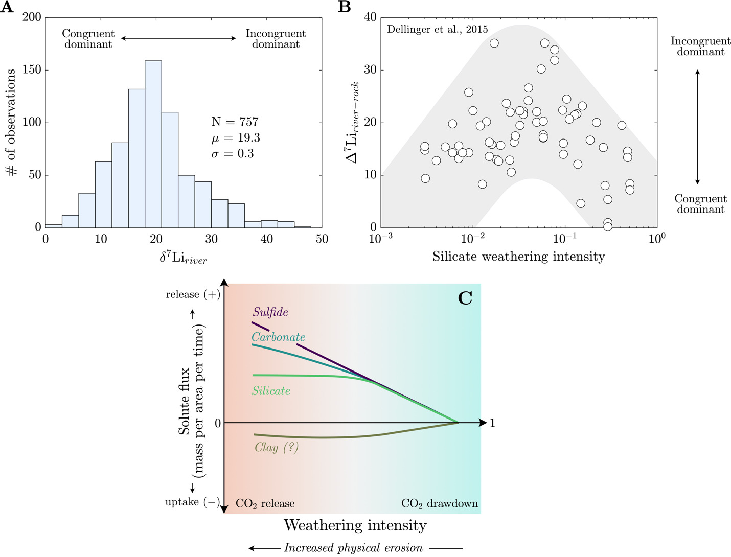
Stable lithium (Li) isotope measurements (δ7Lisample = (7Li/6Li)sample/(7Li/6Li)LSVEC-1; Flesch et al., 1973) of river water and river Li/Na are viewed as complementary and inversely varying indicators of silicate weathering congruency. The rationale for these proxies comes from the abundance and behavior of Li in the weathering environment. Foremost, Li is predominantly found in silicate minerals (e.g. Kısakűrek et al., 2005), with only minor abundances in the carbonate archives used to generate most marine Li isotope records (Kalderon-Asael et al., 2021; Misra & Froelich, 2012). Moreover, Li partitioning and isotope fractionation in weathering environments are largely driven by the formation of secondary clay minerals during the incongruent weathering of primary silicates. During secondary mineral formation, Li favors incorporation into clay relative to other cations, such as Na+ (Bohlin & Bickle, 2019; Tardy et al., 1972), and 6Li is preferentially incorporated over 7Li (Hindshaw et al., 2019; W. Li & Liu, 2022; Pistiner & Henderson, 2003; Vigier et al., 2008; Wimpenny et al., 2010). Lastly, and unlike tracers such as calcium (Ca2+), Li isotopes undergo limited direct fractionation by terrestrial biomass (Clergue et al., 2015; Lemarchand et al., 2010; Pogge von Strandmann et al., 2016; Schmitt et al., 2012). Overall, congruent weathering of silicate minerals generates river δ7Li values and Li/Na comparable to silicate sources. Relative to congruent weathering, formation of secondary clay during incongruent weathering causes δ7Liriver values to increase and river Li/Na ratios to decrease. Together, δ7Liriver values and Li/Na ratios are used to quantify the relative uptake of Li from solution and identify modes of isotopic fractionation at the watershed scale (Bouchez et al., 2013; Dellinger et al., 2015; Georg et al., 2007), offering helpful constraints on the controls of clay formation across the Earth’s surface (e.g., Caves Rugenstein et al., 2019; Dellinger et al., 2015, 2017; Kalderon-Asael et al., 2021; Krause et al., 2023; Misra & Froelich, 2012; Pogge von Strandmann et al., 2020).
The high relative mass difference of 7Li from 6Li and the propensity for Li incorporation into secondary clay minerals generates a globally wide range of δ7Liriver values (Tomascak et al., 2016; fig. 1A). The competing explanations for this wide range of δ7Liriver values reflect the many of the known modulators of chemical weathering at the Earth’s surface: tectonics (Misra & Froelich, 2012; Pogge von Strandmann & Henderson, 2015), climate (Dosseto et al., 2015; Murphy et al., 2019; Pogge von Strandmann, Vaks, et al., 2017; Ramos et al., 2022; Ryu et al., 2014; F. Zhang et al., 2022), bedrock lithology (Dellinger et al., 2015; Henchiri et al., 2016; Pogge von Strandmann, Vaks, et al., 2017; Winnick et al., 2022), physical erosion (Bouchez et al., 2013; Pogge von Strandmann & Henderson, 2015; Winnick et al., 2022), and fluid residence time (Golla et al., 2022; Gou et al., 2019; Henchiri et al., 2016; Liu et al., 2015; Maffre et al., 2020; Manaka et al., 2017; Meier et al., 2017; Wanner et al., 2014; Winnick et al., 2022). Consequently, there is a need to refine the environmental and geologic conditions under which distinct controls regulate Li isotope ratios.
Competing hypotheses exist for how δ7Liriver values, and plausibly seawater δ7Li values, relate to atmospheric pCO2. Reactive transport models of silicate weathering show that δ7Liriver values positively correlate with alkalinity generation via weathering but that fluid residence time and clay Li partition coefficients or fractionation factors can modify the correlation (Wanner et al., 2014). However, these models exclude other, non-silicate phases that would affect the balance of ALK and FIC generation during weathering reactions. In contrast, Li-isotope-based assessments of silicate weathering congruency across climate perturbations often contend that increased clay formation, and thus increasing δ7Liriver values, correspond with greater Ca2+ and Mg2+ uptake and alkalinity consumption that suppress the degree of weathering-driven atmospheric CO2 drawdown (Krause et al., 2023; Pogge von Strandmann et al., 2020). A key focus of this study is clarifying how changes in δ7Liriver are related not merely to silicate weathering and clay formation, but to broader coherent shifts in the ALK and FIC fluxes associated with chemical denudation.
Dellinger et al. (2015) established the current interpretive paradigm of river Li isotope ratios. In their survey of large rivers, Dellinger et al. (2015) showed that δ7Liriver values increase and then decrease with increasing values of silicate weathering intensity (fig. 1B), where silicate weathering intensity is defined as the mass ratio of a watershed-scale chemical silicate weathering flux (mass per area per time) over the sum of chemical silicate weathering flux and total physical erosion fluxes of all sediment (mass per area per time), including non-silicates (Bouchez et al., 2014; eq 6). Comparable weathering intensity indices can be defined for carbonate, sulfide, and clay phases (fig. 1C).
Silicate weathering intensity= (chemical silicate weathering fluxchemical silicate weathering flux+ total physical erosion flux)
There are scenarios where this definition of silicate weathering intensity may be prone to error, e.g., when the abundance of silicate sediment is low, and that this variable does not include the chemical flux due to weathering of carbonate or evaporite materials. However, this formulation has proven useful for characterizing modes of landscape denudation (Bouchez et al., 2014). Empirically, silicate weathering intensity correlates with changes in δ7Liriver values that are thought to showcase limitations of silicate weathering (Dellinger et al., 2015). Specifically, low and high silicate weathering intensities are marked by low δ7Liriver values due to greater proportions of congruent weathering whereas watersheds with intermediate weathering intensities contain notably higher δ7Liriver values due to incongruent weathering. Low δ7Liriver values at low silicate weathering intensities are thought to showcase the kinetic limitation of silicate weathering whereas low values at high silicate weathering intensities reflect dissolution of secondary clay minerals (Henchiri et al., 2016; Winnick et al., 2022). There is less consensus on the processes that undergird the local maxima in δ7Liriver values at intermediate weathering intensity (Deng et al., 2022; Golla et al., 2021; Gou et al., 2019; W. Li & Liu, 2022; Maffre et al., 2020; Pogge von Strandmann et al., 2023; Winnick et al., 2022; J.-W. Zhang et al., 2022) and whether the high δ7Liriver values are strictly associated with landscapes experiencing intermediate silicate weathering intensities (e.g., Golla et al., 2022, 2024; Gou et al., 2019; Pogge von Strandmann et al., 2023). This relationship between δ7Liriver values and silicate weathering intensity has been useful for reconstructing silicate weathering intensity from marine δ7Li records (e.g., Caves Rugenstein et al., 2019). However, beyond the difficulties imposed by the non-uniqueness of the δ7Li-weathering intensity relationship (fig. 1B), maximizing the utility of this relationship necessitates an accounting of all major ALK- and FIC-altering weathering reactions (fig. 1C) involved in or accompanying Li isotope transfer.
In this contribution, we compile a global dataset of published Li isotope river water samples and accompanying solute data and drainage catchment properties. We then calculate the solute sources and sinks for each sample to derive weathering-related ∆ALK/∆FIC and evaluate the capability of weathering-sensitive proxies (δ7Liriver values, river Li/Na ratios) to predict the impacts of chemical weathering on atmospheric pCO2. We focus our attention on river solute chemistry given the significant influence of riverine inputs on marine chemistry (e.g., Coogan & Dosso, 2026). While beyond the scope of this study, we acknowledge that other reactions that occur in estuaries and along coasts (e.g., oxide formation, carbonate precipitation) may alter the net ALK or FIC flux to the ocean (Trapp-Müller et al., 2025). Nevertheless, the drainage catchment properties associated with each river sample allow us to demarcate the environmental and geologic conditions where Li-based proxies are most reliable and draw general relationships between catchment properties and chemical fluxes during chemical weathering. Through these analyses, we identify the outsized influence of bedrock type and climate in describing the range of observed δ7Liriver values and predicted carbon fluxes. We conclude by highlighting areas of improvement in our understanding of continental weathering and the role of clay formation in global element cycles.
2. METHODS
2.1. Overview of global river lithium chemistry database
2.1.1. Data compilation
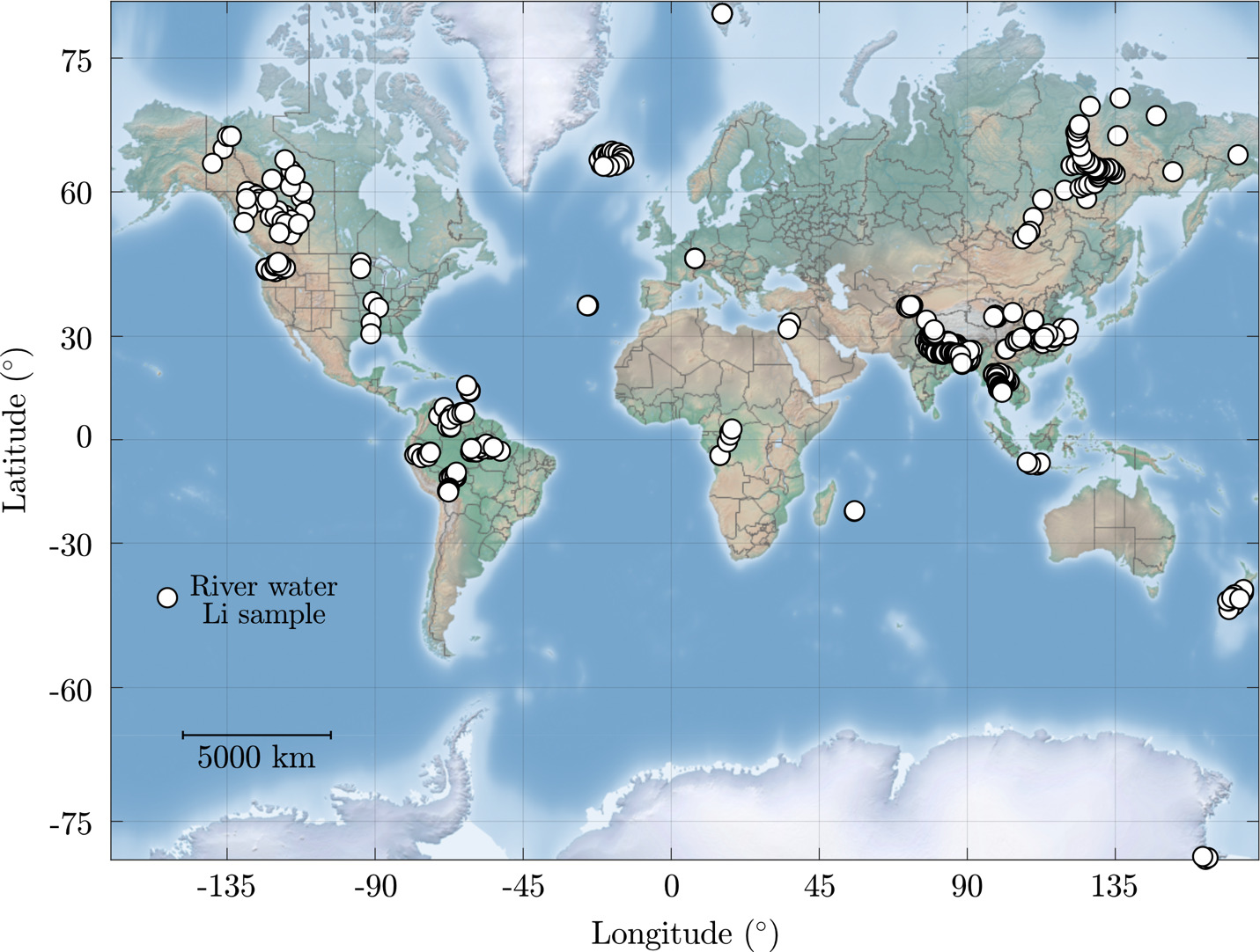
We compiled a global dataset consisting of 757 published δ7Liriver values from 27 studies (table 1; fig. 2). A subset of the data includes river dissolved Li+ concentrations (n = 737), a lesser number of samples (n = 574) report dissolved Li+ and Na+ concentrations, and an even smaller group report anion (SO42- and Cl-) concentrations (n = 413). The sample set includes rivers in all climate zones, draining a wide range of bedrock types, and flowing through a variety of geomorphic settings. Most samples come from well-studied pan-continental river systems with a smaller number of samples from Critical Zone observatories or smaller streams. Data from dry or seasonally wet climates, from Africa, Europe, and the southern hemisphere are underrepresented. On average, the river water samples come from sedimentary rock-dominated catchments with moderate relief and temperate climates, characteristic of most environments presently at the Earth’s surface (fig. 2). Due to gaps in geospatial data around polar regions, we do not include samples from Antarctica (Witherow et al., 2010). Water Li isotope ratios reflect the input of Li through silicate weathering, meteoric precipitation (e.g., Pogge von Strandmann et al., 2006), hydrothermal fluids (e.g., Rad et al., 2013; J.-W. Zhang et al., 2022), evaporites (e.g., Dellinger et al., 2015), and anthropogenic activities including agriculture (e.g., Choi et al., 2019; Millot & Négrel, 2021). Most studies report δ7Liriver values without correction for non-silicate Li input (n = 699, or 92% of all samples), although many studies contend that non-silicate inputs negligibly impact δ7Liriver values. When available, we compile measured δ7Liriver values along with δ7Liriver values that have been corrected for non-silicate inputs. We further address the input of Li from multiple (non-anthropogenic) sources with a river solute inversion technique (see section 2.3). Lastly, few studies in the compilation contain time series of δ7Liriver values from a given location, though the part of the hydrograph that the samples come from are inexact. Typical variability of δ7Liriver values over changes in hydrograph is around 3‰ (Golla et al., 2022; Gou et al., 2019).
_in_this_com.png)
2.1.2. Calculation of δ7Lirock values
Given that different bedrock types can exhibit a >20‰ range in δ7Li values (Tomascak et al., 2016) while individual mineral separates from a given rock can span a >10‰ range (Chapela Lara et al., 2022; J.-W. Zhang et al., 2021), it is important to constrain δ7Lirock values specific to each water sample or locality. We thus adjusted measured δ7Liriver values to be relative to silicate source rock δ7Li values. Offsets in δ7Li values from source rock are presented as Δ7Liriver-rock values (eq 7) defined as
Δ7Liriver−rock= δ7Liriver− δ7Lirock.
We evaluated rock δ7Li values two ways. First, we compiled reported Li isotope composition of river bedload sediment (e.g., Dellinger et al., 2014) or bedrock, which a subset of water samples are paired with (n = 596). We do not consider reported river suspended load δ7Li values because suspended sediment often contains weathered sediment that have δ7Li values less than their source rocks (e.g., Dellinger et al., 2017; Kısakűrek et al., 2005; Lupker et al., 2012). When a range of δ7Lirock values are reported for a given sample set and not explicitly paired with a δ7Liriver value, we compute Δ7Liriver-rock values based on the mean of the reported δ7Lirock values. If no δ7Lirock values are reported (n = 234), we assume a narrow range of δ7Lirock values between +1.0 ‰ and +3.2 ‰, representative of most of the upper continental crust (Sauzéat et al., 2015; Tomascak et al., 2016). Our second method, which serves as a test to the first method, involved computing δ7Lirock values by inverting river solute chemistry for their solute sources (see section 2.3 for more details). The inverted δ7Lirock values were then compared with the bedload/calculated δ7Lirock values and discussed later (see section 4.3). Unless specified, we hereafter present Δ7Liriver-rock values following the first method.
2.2. Determination of drainage catchment properties
Sample locations are crucial for determining drainage catchment geometries. When studies do not report coordinates of sampling locations, we estimated latitudes and longitudes by relating sample location descriptions (e.g., city names, landmarks) and/or map illustrations of sample locations to the largest nearby river reaches in Google Earth®.
We designated individual catchments for each river sample using ArcGIS (ArcHydro tool extension), 30 arcsecond-resolution HYDRO1k global digital elevation data, Flow Accumulation, and Flow Direction rasters (Greenlee, 1987; Jenson & Domingue, 1988; Tarboton et al., 1991; Verdin et al., 2011). The generated watershed polygon was used to extract geospatial information from other global databases including climatic (precipitation and temperature), lithologic (exposed bedrock proportions), and morphometric (mean local relief, mean catchment hillslope angles, and catchment area) information. We refer to these geospatial measurements as catchment properties (table 2).
We derived climate proxies, including mean annual temperature (MAT) and precipitation (MAP) data, from 1 km (~30 arcsecond) spatially resolved and monthly interpolated climate measurements from 1970–2000 included in the WorldClim 2 database (Fick & Hijmans, 2017). These MAT and MAP data do not necessarily correspond to the temperature and precipitation at the time the waters were sampled.
We compiled lithologic data from the 1:3,750,000 area-weighted scale (~1.5 km resolution) global lithology map GLiM (Hartmann & Moosdorf, 2012), which allows for the delineation of contributing surface areas for all lithologic units within each catchment. Of all the units provided, we consider the relative proportions of 12 different rock types including sedimentary rocks (siliciclastic, mixed siliciclastic, pyroclastic, carbonate, and evaporite), plutonic rocks (mafic, intermediate, and felsic), volcanic rocks (mafic, intermediate, and felsic), metamorphic rocks, and unconsolidated sediments in a drainage catchment. The catchment area consisting of glaciers/ice, water bodies, and areas with no data is negligible for all samples. Further, the number of samples with plutonic and volcanic rock-dominated (i.e., proportions ≥ 60%) catchments is small and thus we could not interrogate the differences between felsic and mafic rock-dominated catchments with much statistical significance. All lithologic data for each catchment are presented as proportions. Overall, we find that river catchment lithology is dominated by sedimentary rocks (mean 47%) with moderate proportions (~10–15%) of metamorphic rocks, plutonic rocks, volcanic rocks, and unconsolidated sediment.
Lastly, for morphometric data, we considered catchment area, mean flow lengths, mean local relief, and mean hillslope angles using the 30 arcsecond HYDRO1k digital elevation data (Verdin et al., 2011). Mean local mean relief was computed across the land surface by averaging the elevation over a 3 km-diameter circular area, except for data from Guadaloupe (Rad et al., 2013) that required a 1 km-diameter averaging window due to the demonstrably small area of the island on which samples were gathered. Mean hillslope angles were determined from a study that computed global hillslope angles on a 3 arcsecond DEM (Larsen, Montgomery, et al., 2014). For each sample, we compute a catchment-wide minimum, maximum, mean, and standard deviation for all climatic and morphometric variables.
2.3. Solute inversions with MEANDIR
2.3.1. Solute mixing equations, inversion methods, and model outputs
The MATLAB software Mixing Elements AND Isotopes in Rivers (MEANDIR) from Kemeny and Torres (2021) was used to apportion sources of river solutes, determine weathering acids, and refine endmember compositions. MEANDIR can also account for solute sinks (e.g., clays), which facilitates comparisons of river water Li isotope ratios to clay uptake. River solutes are assumed to be a mixture of solute sources and sinks, mathematically expressed as
(XΣ±)river=N∑jϕj(XΣ±)j
where corresponds to a solute corresponds to a normalization variable that we set to be the charge-equivalent sum of cations and sulfate and corresponds to the fractional contribution of endmember out of a total of N endmembers, to the normalization variable. In this formulation, solute sources have solute sinks have The sum of all fractional contributions to the normalization variable would equal unity if the endmembers could be combined to perfectly describe the data; however, this is rarely possible, and a user-selected degree of calculation misfit determines when a particular inversion attempt is considered to have successfully recreated the observed sample chemistry. Equation (8) can be modified to include Li
(LiΣ±)river⋅((7Li(6Li)river=N∑jϕj(LiΣ±)j ⋅((7Li(6Li)j.
All Li sources are assigned a 7Li/6Li ratio within the range of their a priori distribution whereas clay 7Li/6Li ratios are quantified in accordance with the amount of Li incorporated into clay from solution relative to the amount of Li released from solute sources (Bouchez et al., 2013), shown as
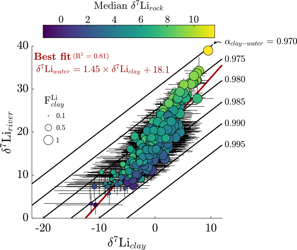
δ7Liriver−δ7Lirock= FLiclayΔ7Liclay−river.
Here is the calculated fraction-weighted δ7Li value of solute sources, is the calculated fraction of Li incorporated into secondary clay relative to Li released by all solute sources, and is an assigned per mil fractionation factor between secondary clay and water. We set a conservatively large range of values (between −30‰ and −5‰; equal to fractionation factor = 0.970 to 0.995, respectively) to encompass the range of reported fractionation factors associated with the Li incorporation into the octahedral, pseudohexagonal, and surface sites of clays (Dupuis et al., 2017; Hindshaw et al., 2019; W. Li & Liu, 2020; Vigier et al., 2008; Wimpenny et al., 2015). The value of is determined by transforming which conveys a fraction of total river solute incorporated from river water into secondary clay, to a value that represent a fraction of Li incorporated relative to gross source input (Cole et al., 2022; Kemeny & Torres, 2021) such that
FLiclay= −ϕLiclay∑NjϕLij−ϕLiclay=−ϕLiclay∑jsourcesϕLijsources.
Equation 11 diverges slightly from the one introduced in Cole et al. (2022) by including the sum of all fractions, in the denominator, which accounts for inversion error in reconstructing river solute compositions. Although expressed for Li uptake, equation (11) is generalizable for the fractional uptake of any solute by clay and all major solutes relative to gross source inputs, with the latter utilizing (see eq 30 of Kemeny & Torres, 2021).
For each river sample, a system of linear equations (eq 8 for each solute and eq 9 for δ7Li) is solved iteratively with a Monte Carlo approach (Kemeny & Torres, 2021). At the beginning of each iteration, random values of each ratio and are drawn from uniform distributions for N-1 endmembers. The normalized ratios for the Nth endmember are then calculated by mass balance and, if its value is negative, the process is repeated. Solutes that are not included in (i.e., Cl-) can have values greater than 1. Once an internally consistent and physically realizable combination of endmember compositions are drawn, a user-specified cost minimization function (we use the function fmincon() in MATLAB) returns optimized values of for each endmember. We only accepted the solution if the returned fractional contributions reconstruct observed solute concentrations and Li isotope ratios within 15% and 5‰, respectively. This procedure is repeated for each sample until either 200 acceptable inversion solutions are found or until 5,000 total iterations have been attempted. The accepted inversions for a given sample are thus composed of a distribution of and for each endmember.
We run two inversions: one without a hydrothermal fluid endmember, referred to as the “base” inversion, and one with a hydrothermal fluid endmember, referred to as the “base + hydrothermal” inversion. In each inversion, at least 99% of all samples were able to achieve at least 1 acceptable inversion solution. The median number of acceptable inversions was 200 for both inversions, but the inversion with a hydrothermal fluid endmember yielded a higher proportion of samples with 200 acceptable inversions (85% vs. 59% in inversion without a hydrothermal endmember). All the statistics regarding the inversion performances can be found in the Supplementary Information (table S.2).
2.3.2. Endmember selection and definitions
The solute sources we consider in our inversion are carbonate, evaporite, silicate, sulfide, precipitation, and hydrothermal fluids, and the solute sink we consider is clay. All endmember bounds are chosen to encompass the broadest ranges of their chemical compositions as to be best applicable to a global compilation of river solute chemistry (table 3). The application of such “global” endmember definitions to small, individual catchments can sometimes lead to errors compared to inversion results employing a larger number of geochemical constraints and/or more local information (Cole et al., 2022; Moore et al., 2013; Torres et al., 2016). As such, future studies building off this work may find slightly different source apportionments at individual sites. However, by purposefully picking wide a priori bounds, we hope that the “true” answer will be encompassed within our estimated uncertainty, which can be the case when comparing inversion models with different numbers of observational constraints (Cole et al., 2022). Ultimately, using a set of broad, shared endmember definitions is useful for our present work in that we wish to highlight differences driven by the observations themselves as opposed to catchment-by-catchment choices for different endmember ranges.
For the carbonate, evaporite, and silicate endmembers, we define endmember bounds for Ca2+, Mg2+, Na+, and Cl- in accordance with previous global river studies (E. K. Berner & Berner, 2012; Burke et al., 2018; Gaillardet et al., 1999; Lerman et al., 2007; table 3). The endmember bounds of major solutes (Ca2+, Mg2+, Na+, Cl-, SO42-) for precipitation is of seawater, following previous inversions of global river solute sources (Gaillardet et al., 1999). We approximate crustal sulfide as pyrite (FeS2) and thus this endmember contributes solely SO42- to river solutes (SO4/ = 1). Evaporites and precipitation are the only other endmembers which contain SO42-. The endmember bounds for Li sources follow observed ranges (Dellinger et al., 2015; Kısakűrek et al., 2005; Pogge von Strandmann et al., 2006; Tomascak et al., 2016; Wang et al., 2015) with predominantly silicates and secondarily evaporites as hosts of Li. We assume the maximum Li content of precipitation corresponds to the Li concentration in seawater (~26 µmol/L or Li/ = 10-5; Broecker & Peng, 1982). We note that our a priori bounds for silicate δ7Li values are broadly defined to account for wide reported ranges for different bedrock types (Tomascak et al., 2016) and among different silicate minerals (J.-W. Zhang et al., 2021).
Hydrothermal fluids have been shown to impact the δ7Li value of river water, especially in headwater catchments and catchments associated with orogenesis, volcanism, or rifting (Henchiri et al., 2014; J.-W. Zhang et al., 2022). The chemical composition of hydrothermal fluids is inherently broad (Giggenbach, 1988) and can itself be viewed as a mixture of solutes sourced from high-temperature fluid-rock interactions. These attributes impose challenges in defining a strict endmember and thus we opt to define them broadly based on observations of thermal springs and outflows reported in previous studies (Giggenbach, 1988; Helper et al., 2023; Henchiri et al., 2014; J.-W. Zhang et al., 2022). In particular, note that our hydrothermal fluid endmember allows Li/ value as high as 0.1, as seen in deep continental brines and hydrothermal systems associated with active orogens (Helper et al., 2023; J.-W. Zhang et al., 2022).
For the clay endmember, we impose a range of Ca2+/ Mg2+/ and Na+/ contents that span the stoichiometric range of different clay mineral types. For example, kaolinite (Al2Si2O5(OH)4) represents cation X/ values equal to 0 whereas smectite ((Na,K,Ca)0.3(Al,Mg)2Si4O10(OH)2·H2O) contain cation X/ values typically between 0.1 to 0.4. Na+/ is nominally lower than ratios for alkaline metals as clays tend to have lower alkali metals contents. Although we acknowledge the discrepancy between Li partition coefficients that are empirically derived ~103 to 106 ppm clay/ppm water; Bohlin & Bickle, 2019) and experimentally derived from clay precipitates (e.g., ~100 to 102 ppm clay/ppm water; Decarreau et al., 2012), we choose Li+/ values that encompass the maximum observed ranges of clay and river sediment (Bohlin & Bickle, 2019; Tardy et al., 1972; Tomascak et al., 2016).
2.3.3. Quantifying rock-derived Li uptake during clay mineral formation
Since the inversions return endmember compositions for each river sample, we can quantify a variable that conveys the relative uptake of rock-derived Li by clay minerals during formation (sometimes referred to as the fraction of Li remaining in solution). Although quite similar to differs in that it considers Li sourced strictly from lithologic sources whereas considers the gross Li from all endmember sources. Isolating the inputs from lithologic sources helps identify the magnitude of rock-derived solute uptake by clay, which is necessary for understanding Li isotope partitioning during rock weathering (Bouchez et al., 2013). We calculate for each sample by first quantifying meteoric-precipitation-corrected solute contents (indicated by an asterisk *) where for a given solute (normalized by the charge-equivalent sum of cations and sulfate; units of Eq/Eq), the precipitation-corrected solute concentration is found as such:
X∗river=Xriver(ϕXsilicate+ ϕXcarbonate+ ϕXevaporite+ ϕXsulfideϕXsilicate+ ϕXcarbonate+ϕXevaporite+ ϕXsulfide+ ϕXprecipitation)
To determine the average bedrock concentration of the solute for a corresponding river sample, where bedrock is defined as a combination of all considered rock endmembers, we perform a weighted average of the inversion-constrained endmember abundance of (normalized by the charge-equivalent sum of cations and sulfate; units of Eq/Eq) and the fractional contribution of this endmember to river water, shown as
Xrock= XsilicateϕXsilicate+ XcarbonateϕXcarbonate+ XevaporiteϕXevaporite+ XsulfideϕXsulfideϕXsilicate+ ϕXcarbonate+ϕXevaporite+ ϕXsulfide.
With these quantities (eqs 12 and 13) determined for both Li and Na, we can calculate which is simply the quotient on river solute chemistry to bedrock chemistry, expressed as
fLidiss=(Li∗Na∗)river(LiNa)rock.
Overall, high values of indicate low Li uptake into clays (high amounts of Li remaining in solution), while low values of indicate high Li uptake into clays (low amounts of Li remaining in solution; Bouchez et al., 2013; Dellinger et al., 2015; Georg et al., 2007; Millot et al., 2010). The usage of Na as a normalizing quantity follows convention (Dellinger et al., 2015) where the primary advantage of the normalization is to account for any dilution that may occur at a given hydrograph stage. Importantly, this definition of assumes that Li+ and Na+ are equally mobile during mineral dissolution (Pogge von Strandmann et al., 2019) and that Na+ is not incorporated into clay minerals during formation (Dellinger et al., 2015), which are safe, first-order assumptions that are not entirely borne out under certain scenarios (Bickle et al., 2015; Cole et al., 2022). Later in the discussion, we illustrate a way to circumvent this complication that facilitates understanding the underlying drivers of clay Li uptake.
2.3.4. Quantifying the effect of weathering on atmospheric pCO2
By tracking the proportional contribution of silicate weathering, carbonate weathering, sulfide oxidation, and clay formation to river solute chemistry, we can approximate the stoichiometry of weathering reactions that allow us to calculate the burden of the weathering system on ocean-atmosphere ALK, FIC, and thus atmospheric pCO2 (Kemeny, Lopez, et al., 2021; Torres et al., 2016). For instance, carbonate formation, which is the primary FIC sink over geologic time, consumes two units of ALK for every one unit of FIC (∆ALK/∆FIC = 2). Therefore, any combination of weathering reactions that lead to ∆ALK/∆FIC 2 will lead to a net drawdown of atmospheric pCO2 over timescales shorter than that of carbonate compensation (10 kyr) and of carbon cycle perturbations 1 Myr). Moreover, since the modern ALK/FIC ratio of the ocean is approximately equal to 1, weathering that yields ∆ALK/∆FIC between 1 and 2 is interpreted to drive pCO2 values lower on short timescales but higher on geologic timescales. Weathering that leads to ∆ALK/∆FIC 1 will yield a net production of atmospheric pCO2 on short and long timescales (~10 Myr).
We constrain the rocks and weathering acids involved in the watershed-scale reactions by using values from model inversions. The fractions of alkalinity generation/consumption relate to inverted endmember compositions (in equivalents) where and for carbonate, silicate, and clay. This definition of ALK is derived through cation concentrations and on the basis of electroneutrality (Middelburg et al., 2020). Our analysis concerns the proportion of carbonate weathering the proportion of sulfuric acid weathering and the proportion of clay alkalinity consumption which are quantified as
R= ϕALKcarbonateϕALKsilicate+ϕALKcarbonate,
Z= ϕALKsulfideϕALKsilicate+ϕALKcarbonate,
and
L= ϕALKclayϕALKsilicate+ϕALKcarbonate,
respectively (Kemeny, Lopez, et al., 2021; Kemeny & Torres, 2021; Torres et al., 2016). Values of span from 0 to 1 where 0 corresponds to weathering of entirely silicates and 1 corresponds to weathering of entirely carbonates. Values of typically range between 0 and 1 but can be greater than 1 (i.e., ∆ALK/∆FIC < 0) if ALK consumption through sulfide oxidation exceeds ALK production through weathering of silicates and carbonates (Kemeny & Torres, 2021). By extension of these definitions, is equal to the proportion of silicate weathering. If we assume that clay minerals source their solutes predominantly from silicates and carbonates, values of clay alkalinity consumption should generally range from 0 to 1 but theoretically could exceed 1 if clay formation consumed cations sourced from additional endmembers. Together, ∆ALK/∆FIC can be calculated from and (eq 18):
ΔALKΔFIC=2(1−Z−LR).
3. RESULTS
3.1. Catchment properties, weathering proxies, and solute chemistry
3.1.1. Relationships among catchment properties and with weathering proxies
Catchment properties and river water chemistry are reported as mean, median, range, and standard deviation/error (table 2). We find a global mean Δ7Liriver-rock value of 17.9‰ ± 7.2‰ (1σ) with a range of 44.3‰. This mean value is comparable to the per mil fractionation factor between octahedrally-bound Li in clay and water (−20‰ to −15‰; Dupuis et al., 2017; Hindshaw et al., 2019; Vigier et al., 2008). The average river Li/Na is 8.1x10⁻⁴, which is about 10% the Li/Na ratio of the upper continental crust (Li/NaUCC = ~10-2; Rudnick & Gao, 2003; Tomascak et al., 2016). Linear regressions of climate variables (mean annual temperature and precipitation), morphometric variables (hillslope angle, catchment area, mean local relief), and river water chemistry (log10(Li+/Na+), log10(Li+), Δ7Liriver-rock) show some significant linear relationships (fig. S.1). Variables of a given class tend to correlate well with one another; for example, MAT and MAP are well correlated = +0.730) and mean local relief and average hillslope angle are well correlated = +0.935). Concerning solely Δ7Liriver-rock values, we find that no morphometric or climatic variable exhibits a significant correlation with Δ7Liriver-rock values (fig. S.1). That is, neither bedrock composition alone, not the climatic or morphometric variables alone, provide a robust basis for prediction. However, through two-way analysis of variance, a procedure which allows us to include categorical data in the comparison of catchment properties with weathering proxies, we determine that there are statistically significant interaction effects among catchment properties (fig. S.1). An interaction effect means that the combined effect of two catchment properties can explain the variation of river chemistry at the 95% confidence interval. This test reveals that interaction effects between bedrock composition and any other catchment properties can explain the range of Δ7Liriver-rock values. In other words, when a climatic or morphometric variable is considered alongside bedrock composition, Δ7Liriver-rock values are statistically predictable. This finding supports that multiple catchment properties are required to explain drivers of river solute chemistry.
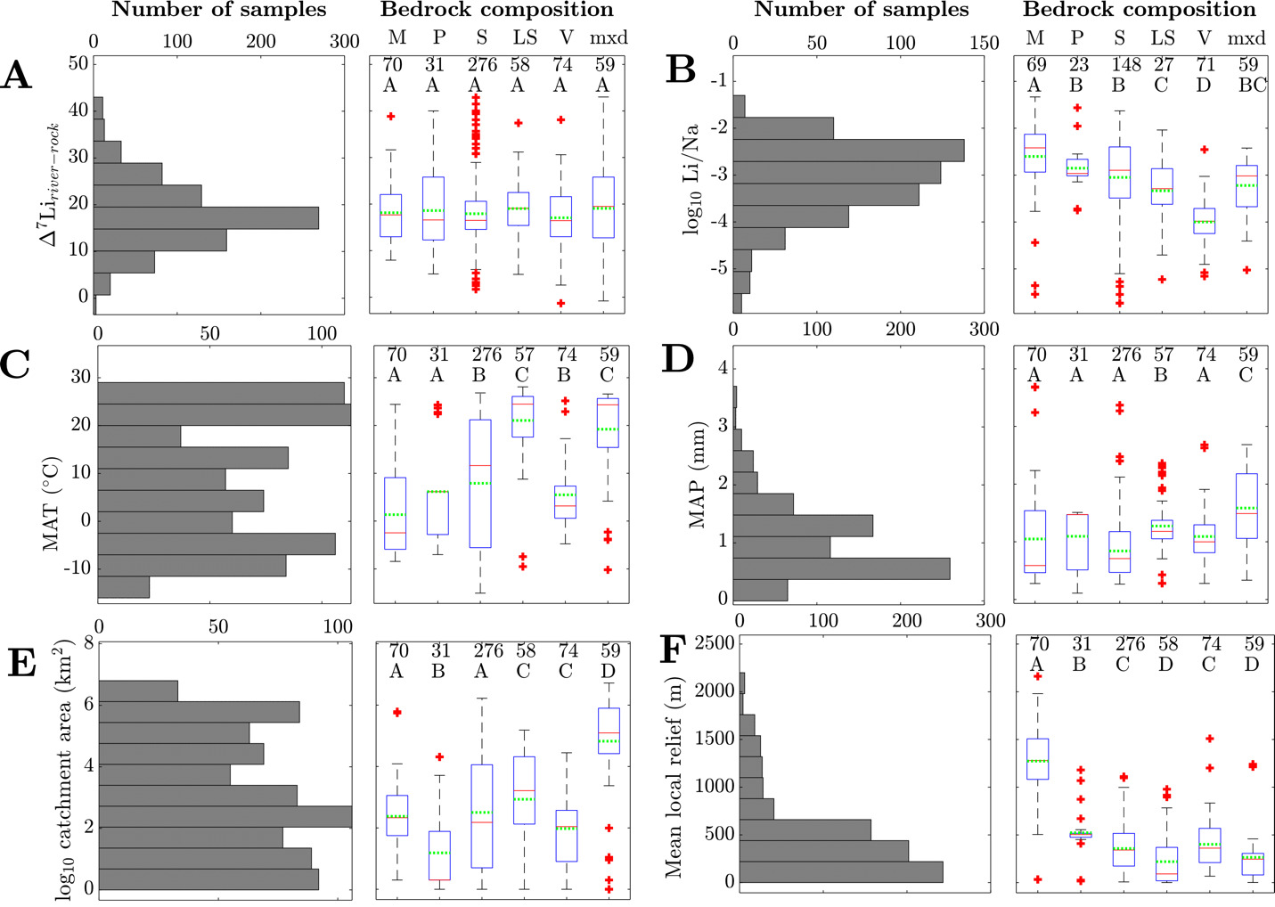
The distribution of weathering proxies, climate variables, and morphometric variables among catchments with variable bedrock composition corroborate the results from the analysis of variance (fig. 3). We discern that the distributions generally fall between two endmember environments that correspond with rock type and physical erodibility. Crystalline rock-dominated catchments, which includes those with a majority of metamorphic and plutonic rocks, tend to comprise small catchments with high relief and low MAT and MAP. Catchments composed of unconsolidated sediments, sedimentary, and mixed bedrocks tend to have larger areas, lower relief, and higher MAT and MAP. The distribution of river log10(Li+/Na+) among different rock-dominated catchments is distinct, with metamorphic rock-dominated catchments having the highest log10(Li+/Na+), volcanic rock-dominated catchments having the lowest log10(Li+/Na+), and sedimentary, unconsolidated sediment, and mixed rock catchments containing intermediate and overlapping log10(Li+/Na+) ranges (fig. 3B). In contrast, the distributions of Δ7Liriver-rock values are indistinguishable among different rock-dominated catchments (fig. 3A). Despite these similarities, the statistically significant interaction effects between bedrock composition and other catchment properties imply that the mechanisms driving Δ7Liriver-rock values in each rock-dominated should differ, potentially related to the associated differences in climate and morphometrics.
__climatic_(c__d)__and_morphometric_(e__f)_catchm.png)
3.1.2. Relationships between major solute chemistry and catchment properties
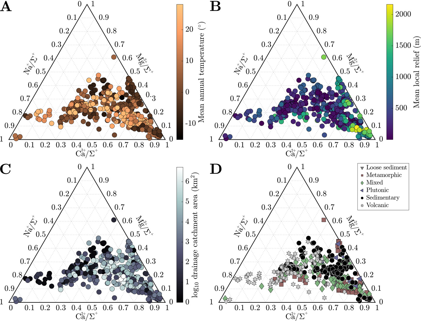
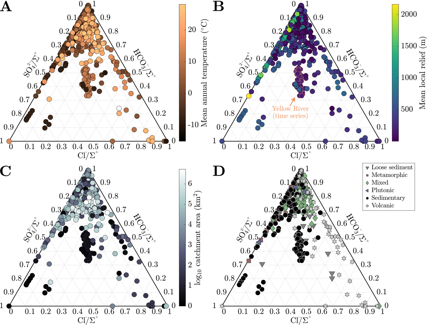
The cation load of most rivers is dominated by Ca2+ (Ca/ = 0.45 ± 0.18), secondarily by Na+ (Na+/= 0.21 ± 0.16), and lastly by Mg2+ (Mg2+/= 0.20 ± 0.08). Cation contents exhibit some general trends among climate, morphometric, and lithologic attributes. Samples with low Na+/ tend to originate in watersheds with low MAT (fig. 4A) and with metamorphic rocks as the dominant rock type (fig. 4D). These same watersheds also tend to have high mean local reliefs and elevated Ca2+/ratios (fig. 4B). Conversely, as Na+/ increases, mean local relief in catchments decreases, MAT increases, and bedrock compositions transition from sedimentary rock-dominates to volcanic rock-dominated at Na+/> 0.6. Mg2+/shows less distinct patterns with respect to MAT and relief, but the samples with the highest Mg content tend to come from metamorphic and plutonic rock-dominated watersheds. Most watersheds of a given rock type have solute chemistry with a narrower range of Mg2+/and exhibit most variability in Ca2+/ and Na+/(fig. 4D). Lastly, as catchment area increases, cation compositions generally become more representative of the compilation average.
._each_point_represents_a_single_samp.png)
We present anion data normalized by the sum of cations where all HCO3- is computed assuming charge balance. SO42-/ Cl-/ and HCO3-/ contrast with cations regarding their relationship to watershed attributes (fig. 5). Across the sample set, HCO3- is the dominant anionic species. SO42-/ has very little connection to climatic or geomorphic attributes of these watersheds. In contrast, Cl-/ most consistently relates to proximity to seawater, with the highest values associated with Icelandic catchments and those at the outlet to the Ganges-Brahmaputra. The smallest drainage catchments almost exclusively have the lowest HCO3-/ (< 0.6) among those in sample set (fig. 5C). Like cations, anions in the largest watersheds are most representative of the compilation average. Although the absolute range of anion contents among the watersheds of a given rock type show substantial overlap, plutonic and metamorphic-rock dominated watersheds tend to have the lowest Cl-/ whereas mixed rock and volcanic watersheds contain water with higher Cl contents. Volcanic watersheds have the narrowest range of SO42-/ ratios, most of which are low in value.
._each_point_is_a_single_sample.png)
3.2. Inversion results
In the following sections, we discuss the major outcomes of the inversions: 1) the fractional contribution of solute sources to river chemistry and weathering-related ∆ALK/∆FIC, 2) the fractional uptake of solutes via clay, 3) the Li isotope expression of clay mineral formation, and 4) the relationships between Li isotope ratios, Li uptake by clay, and weathering-driven ∆ALK/∆FIC. Within each aim, we contextualize inversion results with catchment properties.
3.2.1. Source rock and weathering acid contributions
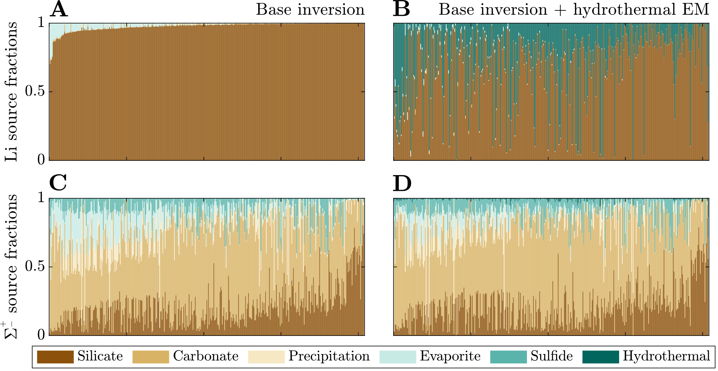
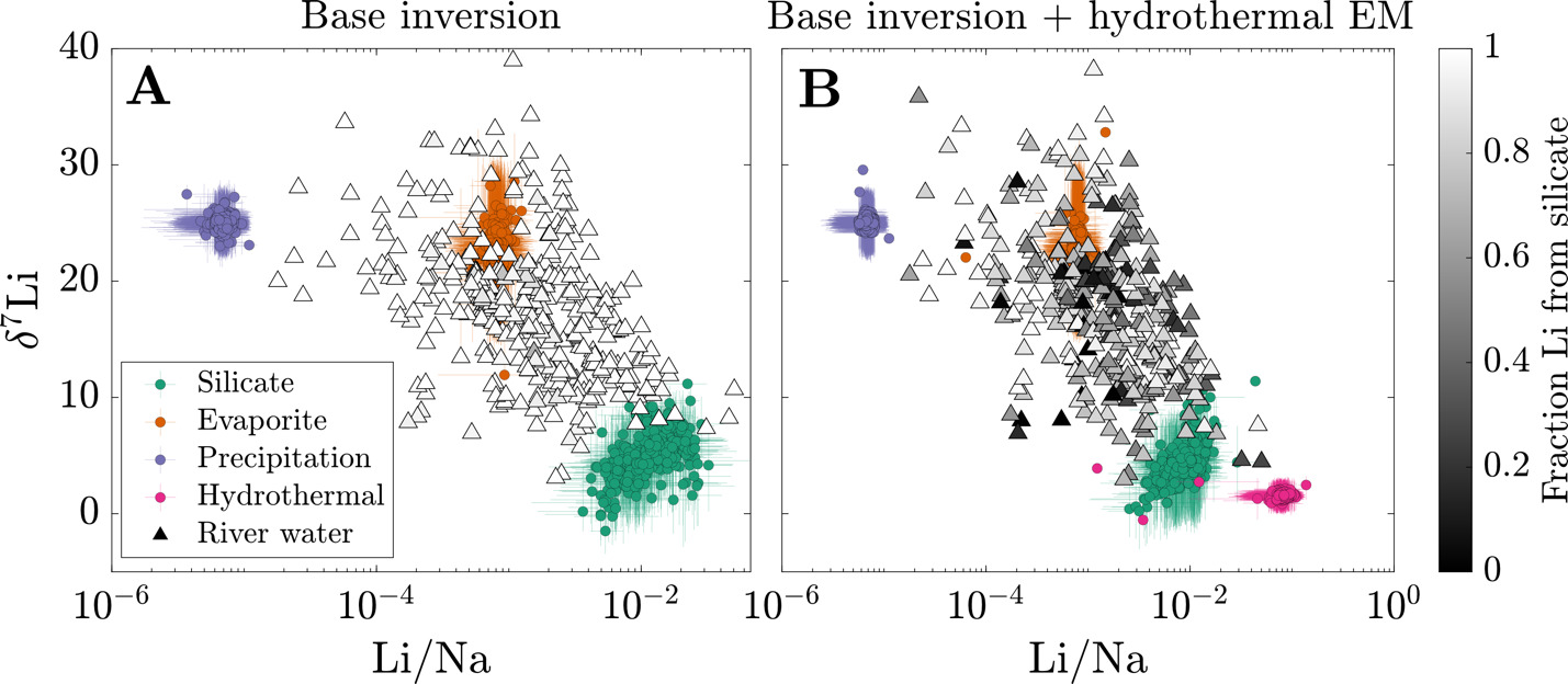
We first focus on the inversion-constrained proportion of each river solute sourced from the different endmembers. To facilitate comparison between samples, we re-normalize the source fractions for each sample such that their sum is equal to 1 (fig. 6). The base inversion predicts that carbonate constitutes the bulk of the solute sources (dataset median = 55 %; IQR = 35 to 67 %) with silicate (median = 19 %; IQR = 10 to 26 %), sulfide (median = 7 %; IQR = 2 to 12 %), evaporite (median = 5 %; IQR = 1 to 15 %), and precipitation (3%; IQR = 0.2 to 11 %) contributing substantially less to samples in the compilation. The tradeoff between silicate and carbonate solute sources is substantial across the sample set = −0.54), and the proportion of silicate-derived solutes tends to negatively correlate with sulfide-derived solute proportions = −0.32). Li+ is predominantly sourced from silicate (dataset median = 98 %; IQR = 96 to 99 %) and lesser amounts evaporite (median = 1 %; IQR = 0.1 to 3 %), but the samples that have > 5% evaporite-derived Li tend to predict higher proportions of bulk solutes derived from carbonate and evaporite.
_and___sigma___pm___(panels_c__d)_from_solu.png)
In comparison to the base inversion, the inclusion of a hydrothermal fluid endmember greatly impacts the relative proportion of Li sources but less so the bulk source contributions. When included in the inversion, hydrothermal fluids are on average the second largest source of Li+ (dataset median = 18 %; IQR = 0.8 to 38 %) and can be responsible for as much as 100% for some samples. Most samples with the lowest Li fractions from silicates tend to be compositionally similar to evaporites (fig. 7), which is most pronounced in the base + hydrothermal inversion but evident also in the base inversion. In general, however, hydrothermal fluids constitute only a small proportion of the net solute budget (dataset median = 0.5 %; IQR = 0.1 to 1 %). That is, while the hydrothermal endmember exerts a large influence on Li specifically, its impact on other element budgets is typically much smaller. As a result, inferences of carbonate weathering fractions and sulfuric acid weathering fractions are consistent between inversions. Values of clay alkalinity consumption fractions generally increase (median increase of 0.07) when a hydrothermal endmember is included, offsetting the additional solutes supplies by the hydrothermal endmember.

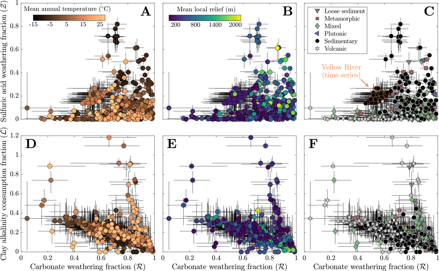
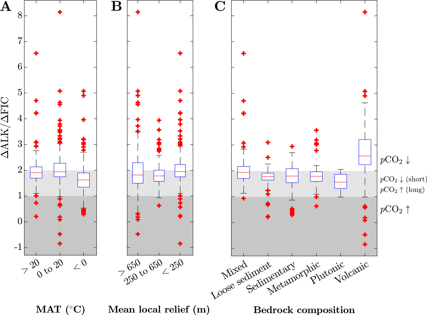
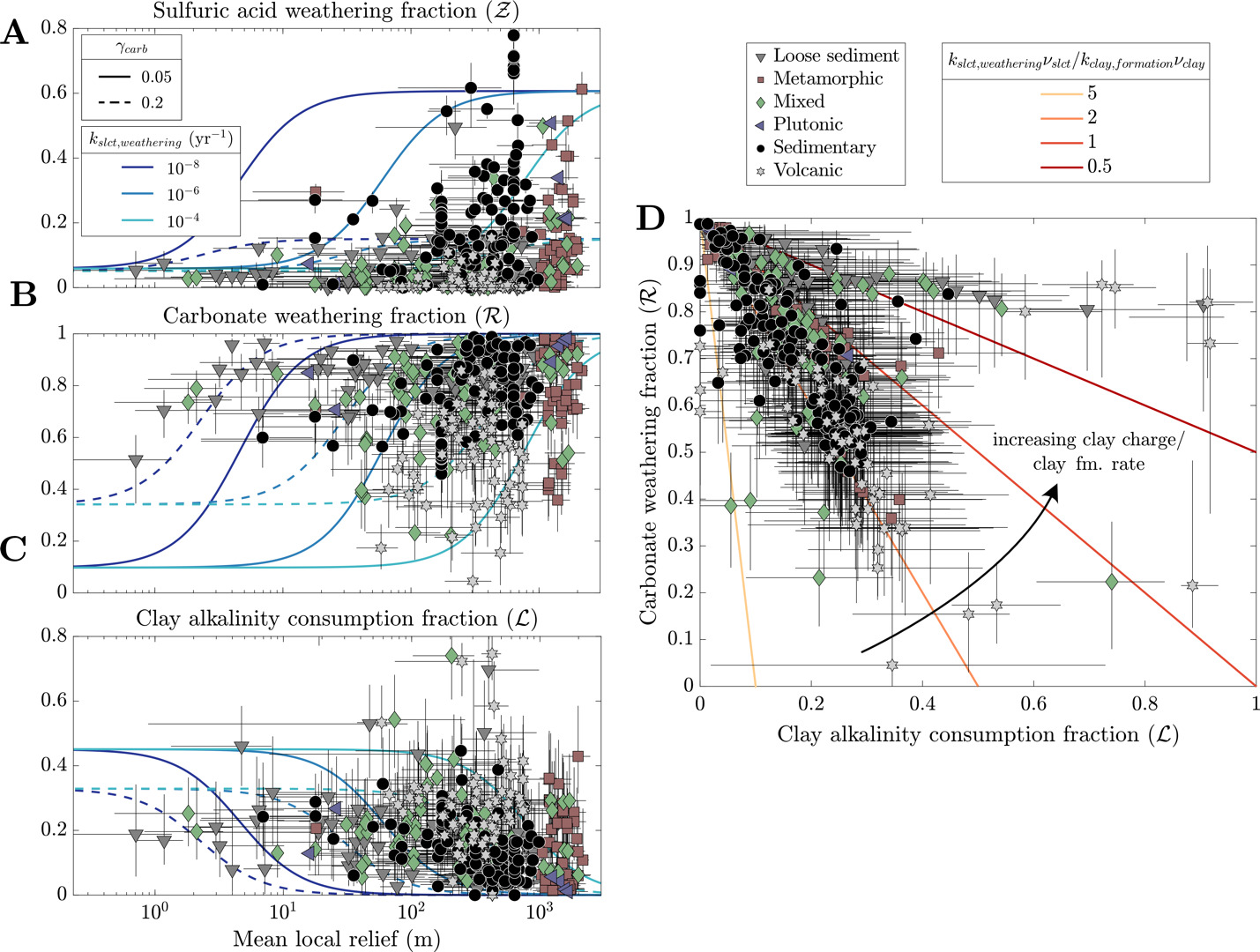
In the base inversion, the range of quantified carbonate weathering fractions and sulfuric acid weathering fractions agree with the range of values from other inversions of global river chemistry datasets (fig. 8; Kemeny, Lopez, et al., 2021; Kemeny & Torres, 2021). Samples with low tend to have low values of but increases in (values > 0.5) correspond with an increase and broadening range of Most samples with low come from watersheds with elevated MAT and MAP regardless of bedrock composition whereas samples with high and high tend to correspond to samples with high mean local relief and either sedimentary or metamorphic bedrock. Nearly all volcanic rock-dominated, whether having low or high MAT, have low The increase in drainage catchment area, and thus a decrease in mean local relief (fig. S.1), is associated with values approaching zero and values approaching 1. Median clay alkalinity consumption fractions span 0 to 1.2 and are weakly correlated to watershed properties (fig. 8D and E). Median values of generally show increases with MAT = 0.19) and MAP = 0.10) and decreases with mean local relief = −0.21). Stronger negative correlations exist with median sulfuric weathering acid fractions = −0.27) and median carbonate weathering fractions = −0.41) but tend not to vary among bedrock types. Volcanic watersheds have the highest median value of 0.28, plutonic watersheds have the lowest median value of 0.05, and all other watershed types have medians ranging between 0.16 and 0.19.
__sulfuric_acid_weathering_(__ma.png)
Together, carbonate weathering fractions sulfuric acid weathering fractions and clay formation fractions determine the ∆ALK/∆FIC ratio of chemical weathering. Median ∆ALK/∆FIC among all samples ranges from −0.8 to +8.1 with a median of 1.9 (fig. 9). In general, as MAT and MAP increase and mean local relief decreases, ∆ALK/∆FIC values increase. However, there is a large amount of scatter in these trends, yielding statistically poor correlations between individual watershed attributes and ∆ALK/∆FIC. Samples grouped according to bedrock type reveal greater distinction in ∆ALK/∆FIC than when climate or geomorphic variables are considered by themselves. Volcanic watersheds have the highest median and widest range of ∆ALK/∆FIC ratio (median ∆ALK/∆FIC = 2.5, absolute range from −0.8 to 8.1) whereas plutonic, metamorphic, and sedimentary watersheds all have narrower and marginally lower ∆ALK/∆FIC (all medians 1.6 to 1.8). Mixed watersheds a have median ∆ALK/∆FIC ratios less than volcanic watersheds but greater than sedimentary, metamorphic, and plutonic watersheds (dataset median = 1.9; IQR = 1.7 to 2.2). Notably, all watersheds grouped according to dominant rock type, climate, and geomorphology have ∆ALK/∆FIC ≤ 1 and > 2, which implies a combination of drivers are responsible for weathering impacts on atmospheric pCO2.
__relief_(b.png)
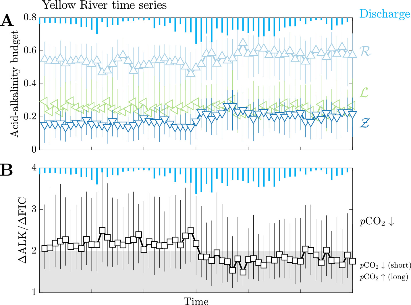
Lastly, results from the Yellow River study (Gou et al., 2019) are shown to convey how changing hydrographs can manifest as changes in rock weathering regimes (fig. 10). We find that median and values change dynamically over a hydrologic year in this locality where carbonate weathering fractions span from 0.46 to 0.65 and sulfuric acid weathering fractions span from 0.14 to 0.27. The standard deviation of median and values among this sample subset is 0.04 and 0.03, respectively, which are values much less than the average interquartile range of and inversion results for samples from this locality (0.27 and 0.19, respectively). Median values vary between 0.20 and 0.31 but do not show systematic changes across the hydrograph. Consequently, the changes of ∆ALK/∆FIC over time largely arise due to changes in the balance of source rocks and weathering acids. The range in magnitude of ∆ALK/∆FIC span from 1.5 to 2.5 across the time series. Both and fluctuate over a hydrologic year, but their mutual increases after peak discharge correspond with a net decrease in ∆ALK/∆FIC ratios from values near 2.4 to values less than 2.
__sulfuric_acid_weathering.png)
3.2.2. Inversion-constrained clay solute uptake
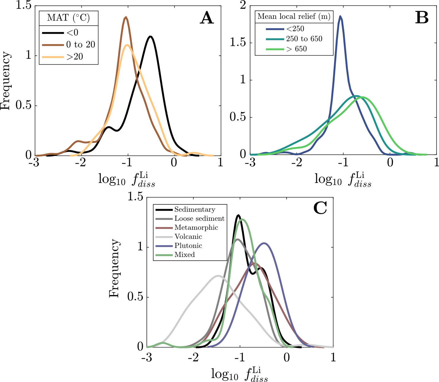
We evaluate the magnitude and drivers of solute uptake via clay, first focusing on non-meteoric Li. The range of values span 3x10⁻³ to 2, with a dataset-median value of 0.12 (IQR = 0.07 to 0.23), corresponding to ~ 88% Li taken up by clay. This median agrees with previous global estimates of amounts of Li uptake via clay formation (~90%; Misra & Froelich, 2012; Tomascak et al., 2016). The distributions of according to MAT shows subtle trends where temperate and tropical watersheds show comparably low and colder watersheds (MAT < 0 °C) have higher values, albeit with substantial overlap. Distributions according to mean local relief are less distinct yet a consistent trend is found. As mean local relief increases (and as MAT accordingly decreases), the distribution of skews toward higher values (fig. 11A and B). Together, these results convey that hotter, flatter watersheds are characterized as ones that uptake higher proportions of Li during clay mineral formation than their cooler, steeper counterparts.
Still larger distinctions among distributions appear when considering dominant bedrock type (fig. 11C). The distribution of values for plutonic watersheds are constrained toward the highest values in the dataset, with metamorphic watersheds showing similarly high values but with a wider distribution of values. Trending toward lower the metamorphic distribution overlaps considerably with sedimentary rock-dominated and mixed watersheds and to a lesser degree with watersheds with primarily loose sediment, which skews toward lower The distinctly lowest values are found among volcanic watersheds whose median value (0.03) is several factors less than any other watershed type (others ranging between 0.10 and 0.32). This demonstrates that Li and Na content of rock cannot alone explain differences in river Li and Na content among the watersheds (fig. S.2); moreover, since watersheds of a given bedrock type span comparable MATs and mean local reliefs, distributions underscore an independent control of bedrock composition on clay formation and Li uptake.

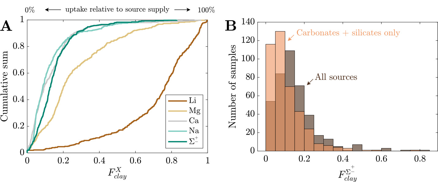
In addition to the uptake of Li+, clays incorporate other cations but to lesser extents (fig. 12A). We now focus on the net fractions of solute uptake relative to source release, which is more pertinent for understanding bulk element mobility and alkalinity consumption. Whereas the dataset-median value is 0.76 (IQR = 0.61 to 0.86), the median values for Na+, Ca2+, and Mg2+ are 0.09, 0.09, and 0.20, respectively. In aggregate, the dataset-median value is 0.13 (IQR = 0.08 to 0.19). The distribution of is opposite those of other elements where the median skews heavily toward high values, and the others element-specific distribution skew heavily toward low values. shows weakly monotonic relationships with and (fig. S.3) where samples with the highest are increasingly likely to have high The groupings of according to among climatic, geomorphic, and climatic groupings overlap considerably (fig. S.3). Whereas clay cation uptake does not appear to be distinct among varying MATs or mean local reliefs, greater (albeit small) contrast is found for clay cation uptake as a function of bedrock chemistry. Of note is the high median for volcanic-dominated watersheds, reinforcing findings of trends among values (fig. 11). We also consider the proportional uptake of silicate- and carbonate-derived solutes by clay to gauge the offset of alkalinity generated by silicate and carbonate weathering during clay formation. These proportions are slightly smaller (fig. 12B); dataset-median values for silicate- and carbonate-derived Na+, Ca2+, and Mg2+ are 0.06, 0.08, and 0.13, respectively, translating to a median value 0.09 (IQR = 0.05 to 0.14). These results show that because silicates and carbonate are the dominant sources of other cations to solution, the solutes clay incorporate from solution will be derived primarily from carbonate and silicates.
_median__f__clay____text_x____values_from_the_base_inversion_presented_as_a_cumulative.png)
3.2.3. The magnitude of Li isotope fractionation via clay formation
We next consider the impact of Li uptake into clay minerals on Li isotope fractionation and evaluate whether bedrock Li isotope ratios are related to fractionation factors. Because the dataset median is about 10 % (or 90 % uptake by clay), we expect clays, as principal Li sinks, to drive Li isotope fractionation. All fractionation factors reflect the difference between inverted δ7Liclay values and inversion-reconstructed δ7Liriver values. The median ∆7Liclay-river value for the entire dataset is −17.9 ‰ (αclay-water = 0.982), with a 25th percentile value of −22.7 ‰ (αclay-water = 0.978) and 75th percentile value of −12.7 ‰ (αclay-water = 0.988). These values agree well with theoretical estimates (Dupuis et al., 2017) and empirical estimates for Li exchange between water and clay octahedral sites (Pistiner & Henderson, 2003; Vigier et al., 2008; Wimpenny et al., 2015). The range of ∆7Liclay-river values are indistinguishable whether the samples are categorically grouped according to MAT, mean local relief, or bedrock type. We also find that inverted δ7Liclay values are mostly insensitive to the inclusion of hydrothermal fluids (fig. S.5), even among inversions where hydrothermal fluids are the dominant Li source. These findings highlight ∆7Liclay-river values as a helpful tracer of Li isotope uptake, even when complicated by hydrothermal fluid inputs (section S.2; figs. S.6 and 7). Lastly, inversions predict median clay Li/ = 0.006 (fig. S.8), near the upper end of our prior range. Translated to a partition coefficient (mass Li clay/mass Li water) by considering the reported river Li/ the compilation median = 29 (IQR = 18 to 47).
We assess that although there is a weakly positive correlation between inverted δ7Lirock and δ7Liclay values, δ7Lirock values show a negative correlation with ∆7Liclay-river values (figs. 13 and S.9). We interpret that this correlation relates to the mutual connection of δ7Liclay and δ7Lirock values to δ7Liriver values via batch fractionation (eq 10). For instance, to satisfy the demand set by high δ7Liriver values, either δ7Lirock values can be high or ∆7Liclay-river values must be very negative (αclay-water < 0.98). Placing a strict, narrow prior range on δ7Lirock values or ∆7Liclay-river values would force the other to change to meet δ7Liriver value constraints during inversions. Across the sample set, the inversion results show that changes in both δ7Liclay and δ7Lirock values are found to successfully reconstruct δ7Liriver values, rather than one of those variables accommodating all the change (fig. 13). These tradeoffs between δ7Liclay and δ7Lirock values to reconstruct δ7Liriver values are not related to the amount of Li supplied by evaporites or hydrothermal fluids either. Rather, these results reflect our broad prior range of δ7Lisilicate values (table 2), beyond those typically considered in global δ7Liriver inquiries and concurrent with mineral-specific δ7Lisilicate values (J.-W. Zhang et al., 2021). Nevertheless, this negative correlation between δ7Lirock values and per-mil fractionation factors agrees with observations of deep regolith (Chapela Lara et al., 2022; Golla et al., 2024) where bulk regolith δ7Li values increase as clay formation continues to enrich pore waters in 7Li.
When grouped according to bedrock type, the distribution of δ7Lirock values show substantial overlap and median values within 3 ‰ of one another (fig. S.10) with plutonic rocks containing the highest δ7Lirock values (median = 7.7 ‰; IQR = 7.1 to 7.9 ‰) and volcanic rocks containing the lowest values (median = 4.2 ‰; IQR = 2.9 to 5.2 ‰). Notably, inverted δ7Lirock values are on average 4 ‰ greater than δ7Lirock values reported or assumed based on bedrock geology (fig. S.10B), potentially supporting the occurrence of 7Li-enriched phases (e.g., feldspar). Consequently, the assumption of δ7Lirock values equal to UCC or another primary geologic reservoir may slightly overestimate the degree Li isotope fractionation.
3.2.4. Clay cation uptake, river δ7Li values, and their comparisons to ∆ALK/∆FIC
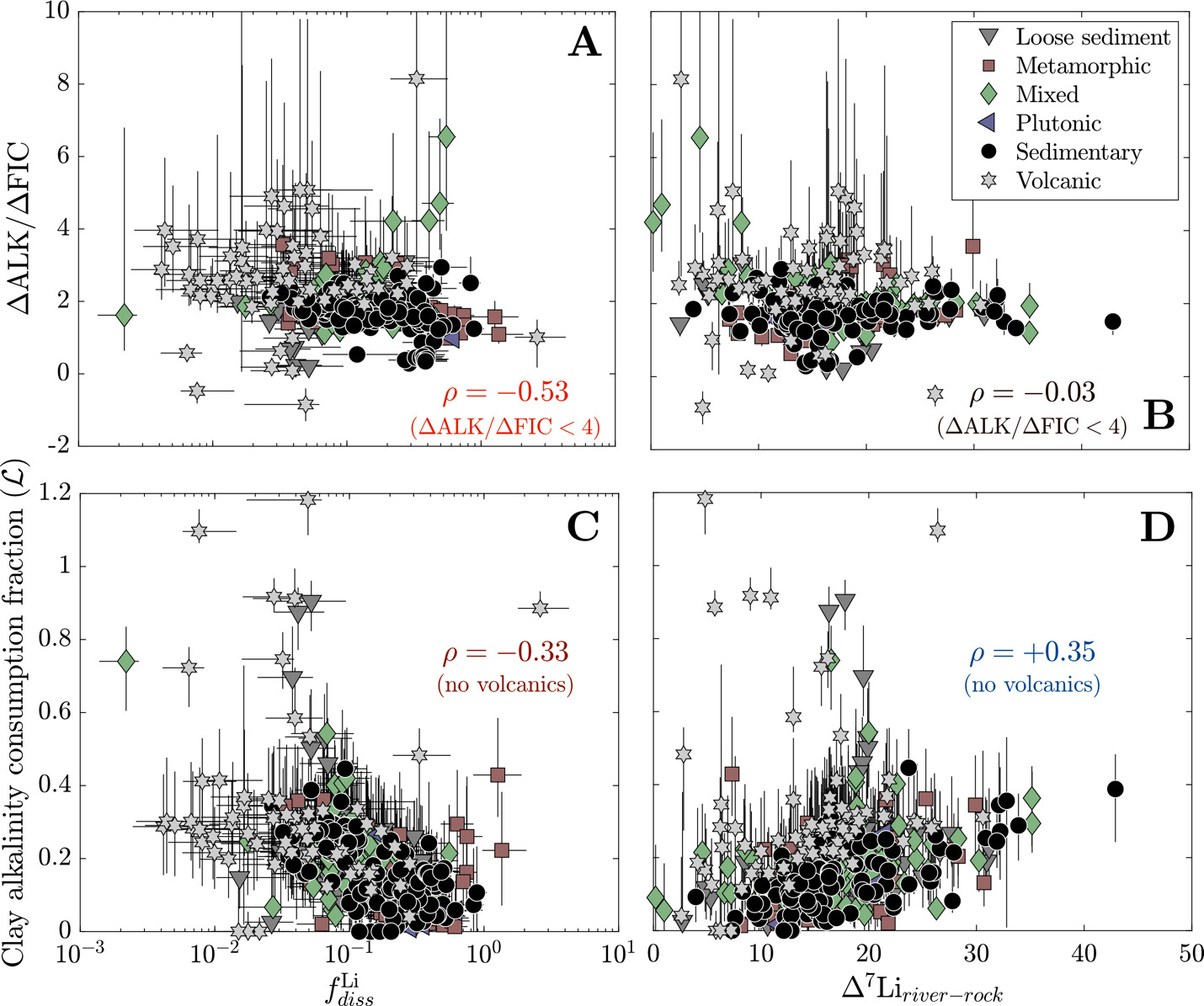
We lastly consider clay cation uptake in the context of river Li isotope ratios and CO2 drawdown. We find that increases in are often associated with increases in ∆ALK/∆FIC, whether considering all solutes = +0.29) or solely those derived from silicates = +0.46). These correlations are echoed in a negative correlation between and ∆ALK/∆FIC = −0.30), a correlation which grows more significant when only considering samples with ∆ALK/∆FIC < 4 = −0.53; fig. 14). Importantly, these correlations hold across different lithologies. In contrast, ∆7Liriver-rock values do not correlate with ∆ALK/∆FIC = −0.09, = −0.03 for samples with ∆ALK/∆FIC < 4) but correlates weakly with clay alkalinity consumption when volcanic watersheds are not considered = +0.35; fig. 14). The Li isotope composition of rivers in volcanic watersheds appear uniquely unrelated to whereas as other rock-dominated watersheds maintain positive correlations whereby higher ∆7Liriver-rock values relate to more alkalinity consumption by clays. Despite clay mineral formation itself reducing alkalinity, overall trends show that as clay minerals incorporate more solutes from water (increasing and less Li remains in solution (decreasing chemical weathering yields an increasing ∆ALK/∆FIC ratio that can decrease atmospheric pCO2. However, river Li isotope ratios only reflect the degree of clay alkalinity consumption and not the net ∆ALK/∆FIC via weathering.

4. DISCUSSION
The inversions show that neither individual watershed attributes such as climate, geomorphology, and bedrock lithology, nor individual weathering proxies such as δ7Liriver values or can alone convey the effects of chemical weathering on atmospheric pCO2. Yet, with sufficient detail about a watershed, assessing the effect of weathering on atmospheric pCO2 and how δ7Liriver values and encodes it becomes increasingly discernible. Here we present a broad investigation of the environmental drivers of weathering and Li transfer across watersheds through derivations of mineral mass balance during rock weathering and by comparison to inversion results. Although discerning the influence of hydrothermal fluids on Li isotope inquiries remains an outstanding challenge, our mass balance model enables us to quantify the sensitivity of river Li isotope ratios to hydrothermal inputs; all discussion on hydrothermal fluids, including model predictions and the inversion results, can be found in the Supplementary Information (section S.2, figs. S.5–S.7). Lastly, to improve the utility of Li isotopes and our understanding of continental clay formation in the geologic carbon cycle, we contextualize our model results by revisiting Li isotope studies of modern watersheds and sedimentary records.
4.1. Regolith mass balance model
4.1.1. Derivation of mass balance equations
The correlation analysis (figs. S.1 and 3), analysis of variance, and inversion results demonstrate that climate, geomorphology, and bedrock types collectively influence chemical weathering and thus river solute chemistry. However, of all the findings, the distinguishable imprint left by lithology on river solute chemistry (figs. 3–9) and (fig. 11) despite the broad range of climatic and geomorphic attributes encompassed in each lithologic group (fig. 3) is particularly noteworthy. The impact of lithology on river solutes is somewhat self-evident since bedrock minerals supply most solutes to rivers. Yet, few studies have explicitly explored the lithologic influence on To understand why lithology has a pronounced impact on Li uptake during clay mineral formation, and how climate and geomorphology may modulate this influence, we derive first-order expressions of mineral mass balance. When comparing model predictions and inversion results, we assume that the mass balance of weathering environments is at a steady state. All variables introduced in our mass balance equations are listed and described in table 4.
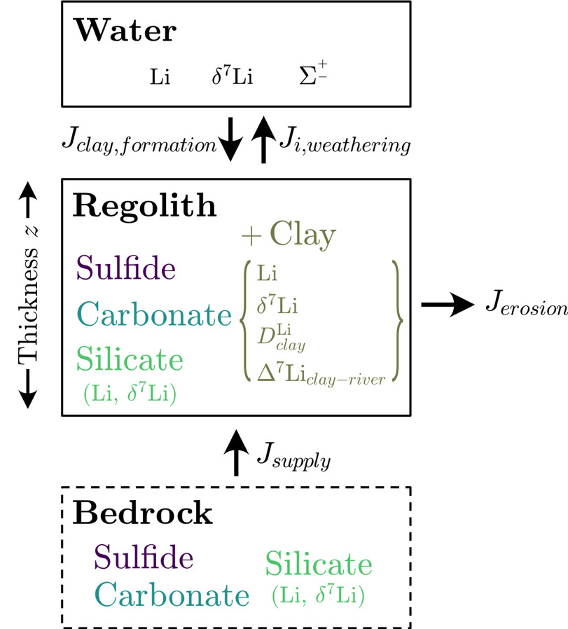
First, in our mass balance equations, we assume a nominal depth in the crust where no weathering is taking place and that overlying this un-weathered bedrock is regolith of a uniform mineralogical composition where weathering is focused (fig. 15). The mass of a given mineral in bedrock and in regolith are defined such that
Mbedrocksilicate+Mbedrockcarbonate+ Mbedrocksulfide=Mbedrocktotal
and
Mregolithsilicate+Mregolithcarbonate+ Mregolithsulfide+ Mregolithclay=Mregolithtotal.
We assume that all clay found in regolith is the byproduct of chemical weathering reactions. We also exclude porosity from our definition of regolith and consider solely the evolution of solid mass. The change over time in the mass of given mineral (subscript in regolith is driven by bedrock fluxes into regolith during uplift units of mass⋅time-1) and output fluxes via physical erosion and chemical weathering expressed as
dMregolithidt=Jsupply−Jerosion−Jweathering =ksupplyMbedrocki−(kerosion+ki,weathering)Mregolithi
Here all terms are rate constants (in units of time-1) and they pertain to the rate of mineral supply from bedrock and the rates of physical erosion and chemical weathering of a mineral in regolith. In soil mantled environments, the supply of bedrock that regulates soil production should be greater than or equal to the rate of erosion under a constant erosional forcing. The net rate of bedrock supply is often framed as the product of an intrinsic rate and a decay constant that describes the decrease of the supply rate with increasing regolith thickness (e.g., Heimsath et al., 1997). If we assume that the distribution of watershed elevations is at an equilibrium state such that denudation equals uplift and regolith thickness remains constant, the mass of a given mineral in regolith will achieve a steady state (Ferrier & Kirchner, 2008; Ferrier & Perron, 2020). In our formulation, we assume that the value implicitly includes this depth dependence and that and are time-invariant.
Setting equation (21) equal to zero following the steady state assumption, we define a steady state mineral mass (denoted with subscript such that
Mregolithi,∞=ksupplykerosion+ ki,weathering Mbedrocki,∞.
For authigenic phases that form in regolith, like clay, their supply is connected to the abundance of its predominant parent phase (silicate). The expression for the mass balance of clay minerals in regolith thus takes the form of
dMregolithclaydt=Jclay,supply−Jclay,erosion−Jclay,weathering=kclay,formation Mregolithsilicate− (kerosion+ kclay,weathering) Mregolithclay.
Here we assume that the amount of clay that forms in regolith is set by the mass of primary silicates in regolith and their rate of mineral dissolution. Furthermore, we distinguish and to capture the potential influence of clay dissolution on Li isotope dynamics (e.g., Dellinger et al., 2015). At steady state, equation (23) can be recast to show the steady-state mass of clay in regolith as a function of steady-state silicate in regolith whereby
Mregolithclay,∞=(kclay,formationkerosion+kclay,weathering)Mregolithsilicate,∞.
Substituting equation (22) for silicates into equation (24) for clay, we find that
Mregolithclay,∞=(kclay,formationkerosion+kclay,weathering)⋅(ksupplykerosion+kslct,weathering)Mbedrocksilicate, ∞.
To evaluate Li uptake in a steady-state weathering environment, we next introduce expressions for the mass balance of Li in clay where
ddt(MregolithclayLiregolithclay)=JLiclay,formation−JLiclay,weathering=kclay,formationMregolithsilicateDLiclayLiwater−kclay,weatheringMregolithclayLiregolithclay.
Here, including a partition coefficient (mass Li clay/mass Li water) assumes a fixed ratio of Li in clay relative to that in water. We can expand the lefthand side of equation (26) using the product rule and substitute equation (23) for the time derivative of yielding an expression for such that
ddt(Liregolithclay)= kclay,formationMregolithsilicateMregolithclay×(DLiclayLiwater−Liregolithclay).
The mass balance of Li in water can be described as
ddt(Mwater Liwater )=JLisilicate,weathering +JLiclay,weathering −JLiclay,formation =ksilicate,weathering Mregolith silicate Lisilicate +⋯kclay,weathering Mregolith clay Liclay,regolith −⋯kclay,formation Mregolith silicate DLiclay Liwater .
Here we assume that Li is introduced into water via the dissolution of primary silicates and clay in regolith and that Li is removed from water via clay mineral formation. The amount of Li incorporated into clay is proportionate to the partition coefficient of Li between clay and water (mass⋅mass-1) and its formation rate For simplicity, we impose a constant Li content for silicate sources If we assume that all solid regolith masses are greater than zero and that the water-rock ratio of the porous regolith is constant at a steady state (i.e., is constant), the steady state value is simply
Liregolithclay,∞=DLiclayLiwater∞.
Moreover, solving equation (28) for a steady state composition returns
Liwater∞=ksilicate,weathering Mregolithsilicate,∞Lisilicate+ kclay,weathering Mregolithclay,∞Liregolithclay,∞kclay,formationMregolithslilicate,∞DLiclay.
By substituting equations (25) and (26) into (27), we arrive at a simpler expression for wherein
Liwater∞=ksilicate,weathering LisilicateDLiclaykclay,formation×(1− kclay,weatheringkerosion+kclay,weathering).
If we lastly normalize equation (31) by and rearrange it, we arrive at a new and complementary expression for a steady state :
fLidiss∞=(ksilicate,weatheringDLiclaykclay,formation)(kerosion+ kclay,weatheringkerosion).
It is noteworthy that is not a function of nor because each flux that constitutes equation (28), at a steady state, is proportionate to this mass. Instead, equation (32) demonstrates that is a function of two dimensionless ratios: one that conveys the balance of Li supply from silicate dissolution and Li uptake via clay formation and another that conveys the relative rates of bedrock mineral supply and secondary clay dissolution.
4.1.2. Estimating rate constants for mass balance equations
We now make several assumptions regarding the values and definitions of the corresponding rate constants in equation (32). Using an Arrhenius dependency, the chemical weathering rate constant for mineral depends on its intrinsic (far-from-equilibrium) rate constant (time-1), the difference between weathering temperature (K) and reference temperature (K), phase-specific activation energy (kJ mol-1), and the departure from equilibrium related to water infiltration rate (length⋅time-1) such that
ki,weathering= ki,intrinsice(EaiRT0−EaiRT)(1−e−0.06×q).
Equation (33) assumes that the approach to equilibrium is set by the residence time of fluid flowing where as (Maher, 2010). The constant value (time⋅length-1) is empirically derived from laboratory- and field-derived silicate weathering rates (Maher, 2010). For simplicity, we assume that the fluid-residence-time dependence applies equally to all phases, although its influence on carbonate and sulfides is minimal due to their high rate constants (Bufe et al., 2021). To assess the sensitivity of to variations in and for samples in our compilation, we use watershed MAT and MAP for each sample as measures for and respectively, and calculate the range of : ratios considering the range of values for major rock-forming minerals (25 to 60 kJ/mol). We calculate the sensitivity of to the combined effect of temperature and infiltration maximally ranging 2.7 orders of magnitude. In contrast, values of are vastly different among sulfide, carbonate, silicates, and clay, up to 6 orders of magnitude in absolute range (Palandri & Kharaka, 2004; White & Buss, 2014). Thus, while climate variables meaningfully impact rock weathering rates, the distribution of mineral types, and thus lithology, is the likely discriminating factor among drivers for samples in our compilation.
Second, we determine values for through its connection to mean local relief (Ludwig & Probst, 1996; Montgomery & Brandon, 2002). We use the empirical power law relationship between relief and physical erosion of Montgomery and Brandon (2002) which is described as
E= aSb
where the physical erosion rate (mm⋅yr-1) correlates with mean local relief (m) and is modified by empirical constants (equal to 1.4 10-6) and (equal to 1.8). This relationship is relevant to regions of active orogenesis and derived from observations of mean local relief spanning those of watersheds in our compilation. To relate to we lastly assume a weathering zone thickness (mm) such that
kerosion= Ez=aSbz.
The thickness of the weathering zone is thought to vary in conjunction with relief (e.g., Ferrier & Kirchner, 2008; Heimsath et al., 1997; Larsen, Almond, et al., 2014) assuming that soil is the sole locus of chemical weathering. However, it is shown that weathering zone thicknesses extend farther into fractured bedrock (Golla et al., 2021; Moon et al., 2017; Tune et al., 2020) and possibly to depths equivalent to mean local relief (L. Li et al., 2018; West, 2012). In subsequent analyses we assume a nominal weathering zone thickness of 1 m for all samples, but we acknowledge that values of can modulate values of and other modeled quantities (see section 4.2) at high relief (fig. S.11). Together with equation (32) and (35), the complete equation of is
fLidiss∞=(ksilicate,weatheringDLiclaykclay,formation)(kerosion+ kclay,weatheringkerosion)=(ksilicate,weatheringDLiclaykclay,formation)×(1+z kclay,weatheringaSb).
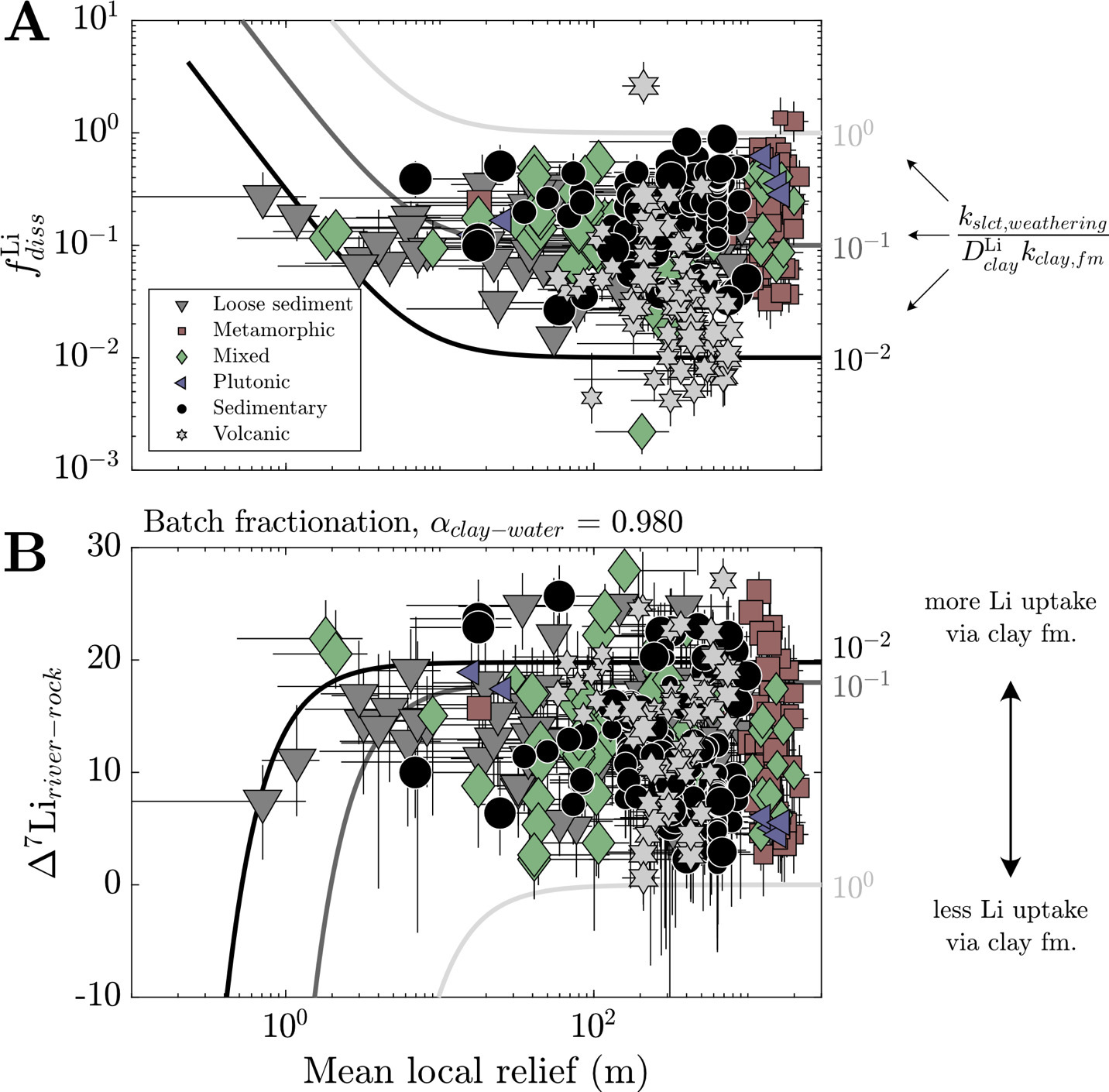
The predictions of as a function of relief reveal key trends (fig. 16A). First, when mean local relief increases, the value will approach the value of This limit suggests that the mineralogical makeup of a rock, with their inherent rates of dissolution and which partly set the products of weathering reactions, governs the value of at high relief. As relief decreases and thus decreases, the value of will increase (fig. 16A), corresponding to less clay formation. The rate of increase with decreasing relief depends on the value of where higher values of will cause swifter increases in with decreasing relief (fig. S.12). This relationship makes sense because if clay minerals are dissolving faster than fresh bedrock silicates are being supplied, there should be high relative amounts of Li remaining in solution. At low relief, high suggests less Li is incorporated in clay minerals. This contrasts with high relief environments where higher relative amounts of Li incorporation into clay. Changes in weathering temperature and infiltration rate will variably influence the values of and impacting and its relationship with relief (fig. S.13). An increase in temperature will increase all these rate constants, causing to increase. In contrast, increases in infiltration forces all rate constants higher but causes greater relative increases in relative to leading to increasing at low relief (< 1m) but unchanging at high relief. The impacts are consistent with observations of Li isotope records across periods of hydroclimate change (e.g., Pogge von Strandmann et al., 2020; Pogge von Strandmann, Frings, et al., 2017; F. Zhang et al., 2022). Over the range of MAP and MAT in the watersheds, MAT has a more sizable impact on Li isotope dynamics than infiltration rate in these steady state calculations (fig. A.13).
__f__diss___li___(fraction_li_remaining_in_solution)_and_(.png)
We can extend this definition of to predict the steady state ∆7Liriver-rock values as a function of mineral supply. Typically, these calculations assume equilibrium Rayleigh or batch fractionation (Bouchez et al., 2013; similar in principle to equation 10), which are expressed as
Δ7Liriver−rock=−1000lnαclay−water(1−fLidiss∞)
and
Δ7Liriver−rock=1000lnαclay−water log(fLidiss∞),
respectively. Although these equilibrium fractionation constructs are not necessarily applicable to individual weathering profiles or flow paths (e.g., Golla et al., 2021), they can be reasonably applied to river water due to the integration of many flow paths within a watershed (Druhan & Maher, 2017). These calculations show that ∆7Liriver-rock values have the opposite of trends with mean local relief (fig. 16B). We note that all solutions here are presented as sensitivity analyses that bracket observations to demonstrate the influences steady-state solutions and how they may be encoded in river chemistry. At low relief, because less Li is incorporated in clay minerals, the corresponding ∆7Liriver-rock values will be low. This contrasts with high relief environments where higher relative amounts of Li incorporation into clay drive ∆7Liriver-rock values higher. The range of ∆7Liriver-rock values will be modulated by where low values, corresponding to high rates of clay mineral incorporation of Li relative to supply from mineral, will increase the maximum achieved ∆7Liriver-rock values. The mode of isotopic fractionation as well as the magnitude of ∆7Liclay-water are also important factors, where Rayleigh fractionation and more negative ∆7Liclay-water fractionation factors generate wider variation of ∆7Liriver-rock values as a function of relief, which may be necessary to explain samples with ∆7Liriver-rock > 25 ‰.
Without invoking other modifications to our calculations, such as changing the fractionation factor αclay-water or the mode of isotopic fractionation, the steady state solutions predicted for and ∆7Liriver-rock can bracket those values determined through the inversion (fig. 16B). Critically, the trends of and ∆7Liriver-rock as a function of relief agree qualitatively with the dominant bedrock types in the watershed and, to a lesser extent, climate. Rocks that undergo rapid chemical weathering at Earth surface conditions and whose secondary minerals incorporate high proportions of Li, like volcanic rocks, tend to have low and vice versa for rocks that undergo less rapid weathering and incorporate less Li, like sedimentary rocks and unconsolidated sediment (fig. 11C). The indistinguishability of ∆7Liriver-rock values across bedrock types (fig. 3A) does not necessarily undercut the role of mineral supply in driving Li isotope fractionation. Instead, it may point to influence of other complicating factors, like partition coefficients, isotopic fractionation factors, and modes of isotopic fractionation that may correlate to changes in lithology. As an example, for weathering of volcanic rocks to yield low ∆7Liriver-rock values given their characteristically low the αclay-water value must be closer to 1, which could be possible if gibbsite is the authigenic phase (e.g., Wimpenny et al., 2010, 2015); this is lent credence by a weak positive correlation between inversion-constrained ∆7Liclay-water fractionation factors and At another extreme, for weathering of unconsolidated sediment to yield high ∆7Liriver-rock values given their characteristically high the αclay-water value must be less than 1 (< 0.98), which could be possible if kaolinite is forming and sorption of Li magnifies isotopic fractionation (e.g., W. Li & Liu, 2020). Less evidence for this exists from our dataset, where the poor correlation between median ∆7Liclay-water fractionation factors and for these watershed types indicates other potential modulators of such as climate.
Altogether, the results of this mass balance model illustrate that the rates of silicate mineral dissolution relative to the rates of mineral supply play a paramount role in the Li isotope composition of river water, aligning with the weathering intensity hypotheses introduced in Bouchez et al. (2013) and Dellinger et al. (2015). However, our model furthers this hypothesis to demonstrate that while climatic impacts may subtly alter ∆7Liriver-rock values, intrinsic weatherability of sediment (set by bedrock lithology) compared to mineral supply more clearly manifests in the broad variability of ∆7Liriver-rock values across all watersheds. Pinpointing how climate and lithology impact river Li isotope compositions will likely require a detailed characterization of secondary clay minerals within a given watershed, since the composition of clay minerals relates to bedrock mineralogy, evolves with climate conditions (Folkoff & Meentemeyer, 1985), and corresponds with varying degrees of Li incorporation and isotopic fractionation (Bohlin & Bickle, 2019; Pistiner & Henderson, 2003).
4.2. Alkalinity generation and the balance of weathering reactions
The countervailing effect of sulfide oxidation on net CO2 drawdown via weathering has received significant attention due to its prevalence in mountainous terrains that are traditionally consider loci of large silicate weathering fluxes (Bufe et al., 2021; Calmels et al., 2007; Kemeny, Lopez, et al., 2021; Torres et al., 2014, 2016). As evidence for ubiquitous sulfide oxidation grows across a wide range of Earth surface environments, it is important now to evaluate where our understanding of Li isotope transfer at the Earth surface intersects with sulfide oxidation. Moreover, an accounting of alkalinity consumed during clay mineral formation has not yet been thoroughly examined beyond a handful of Li isotope studies (e.g., Wanner et al., 2014). Here we demonstrate that sulfuric acid weathering and clay mineral formation are connected by their mutual dependence on mineral supply and physical erosion.
We can express the definitions of the fractions of sulfuric acid weathering eq 16), carbonic acid weathering eq 15), and clay formation fractions eq 17) using mass balance equations. For instance, if we consider the weathering flux of carbonate, silicate, and sulfide minerals, we can recast sulfuric acid weathering fractions such that
Z=νsulfideJsulfide,weatheringνcarbonateJcarbonate,weathering+ νsilicateJsilicate,weathering
which expands to
Z=νsulfideksulfide,weatheringMregolithsulfideνcarbonatekcarbonate,weatheringMregolithcarbonate+ νsilicateksilicate,weatheringMregolithsilicate.
Here the coefficients correspond to the charge of the solutes being generated. Whereas sulfide and carbonate have equal to 2, has a value between 1 and 2 depending on the proportion of alkali and alkaline metals in primary silicates. Thus, if we consider the steady state fraction of sulfuric acid weathering we can substitute equation (22) for each mineral into equation (40) and arrive at an expression that states
Z∞= (ksulfide,weatheringkerosion+ ksulfide,weathering)νsulfideMbedrocksulfide(kcarbonate,weatheringkerosion+ kcarbonate,weathering)νcarbonateMbedrockcarbonate+ (ksilicate,weatheringkerosion+ ksilicate,weathering)νsilicateMbedrocksilicate.
Notably, equation (41) shows that sulfuric acid weathering, at a steady state, should depend strictly on the composition of un-weathered bedrock and not that of regolith (Bufe et al., 2022). We can normalize the numerator and denominator on righthand side of equation (41) by so that is expressed in relative, rather than absolute, mass of minerals, which we denote with the symbol It is expressed as such:
Z∞=(ksulfide,weatheringkerosion+ ksulfide,weathering)νsulfideγbedrocksulfide(kcarbonate,weatheringkerosion+ kcarbonate,weathering)νcarbonateγbedrockcarbonate+ (ksilicate,weatheringkerosion+ ksilicate,weathering)νsilicateγbedrocksilicate.
Equations (35) and (42) can be combined to describe a steady state fraction of sulfuric acid weathering due to mineral supply:
Z∞=(ksulfide,weatheringaSbz+ ksulfide,weathering)νsulfideγbedrocksulfide(kcarbonate,weatheringaSbz+ kcarbonate,weathering)νcarbonateγbedrockcarbonate+ (ksilicate,weatheringaSbz+ ksilicate,weathering)νsilicateγbedrocksilicate.
With similar assumptions, we can arrive at expressions for steady state carbonate weathering fractions which is described as
R=νcarbonateJcarbonate,weatheringνcarbonateJcarbonate,weathering+ νsilicateJsilicate,weathering
in its full form and at steady state, in its reduced form
R∞=(kcarbonate,weatheringaSbz+ kcarbonate,weathering)νcarbonateγbedrockcarbonate(kcarbonate,weatheringaSbz+ kcarbonate,weathering)νcarbonateγbedrockcarbonate+ (ksilicate,weatheringaSbz+ ksilicate,weathering)νsilicateγbedrocksilicate.
The expression for clay alkalinity consumption fraction can be shown as
L=νclayJclay,formationνcarbonateJcarbonate,weathering+ νsilicateJsilicate,weathering
which expands to
L=νclaykclay,formationMregolithsilicateνcarbonatekcarbonate,weatheringMregolithcarbonate+ νsilicateksilicate,weatheringMregolithsilicate
and at a steady state can be shown in its complete form
L∞=(kclay,weatheringaSbz+ ksilicate,weathering)νclayγbedrocksilicate(kcarbonate,weatheringaSbz+ kcarbonate,weathering)νcarbonateγbedrockcarbonate+ (ksilicate,weatheringaSbz+ ksilicate,weathering)νsilicateγbedrocksilicate.
like and is affected by the proportion of bedrock minerals but is additionally sensitive to the balance of rates for clay mineral formation and silicate dissolution. The charge of clay minerals corresponds to a value that is likely less than or equal to and can be as low as 0 if the clay does not contain base cations (e.g., kaolinite).
The results of our sensitivity analyses demonstrate the conditions in which inverted and values agree with model predictions (fig. 17A–C). Like for the steady state Li isotope predictions, we present generic solutions for and that bracket observations to gauge how bedrock composition and silicate/clay rate constants may underlie there chemistry. In general, the dissolution of carbonate and sulfide minerals follow similar patterns whereby mean local relief positively correlates with and Low and are found at low mean local relief until surpassing a threshold relief range where they steeply increase at moderate relief. The threshold relief range is primarily modified by the relative weathering rates of carbonate, silicate, and sulfide, and the magnitude of this increase and the maximum and values at high relief correlate with the fraction of bedrock sulfide and carbonate, respectively. The fractions of sulfuric acid weathering and carbonate weathering decrease with increasing MAT and MAP because the concomitant increases in the rates of carbonate and sulfide weathering consume all available carbonate and sulfide, leaving regolith bereft of these more weatherable phases. Although relying on observations from one hydrograph (Gou et al., 2019), we surmise that mineral supply can be modulated by the transience in subsurface flow whereby the depth of the water table relative to the depths of the carbonate and sulfide reaction fractions will alter the balance of and (Kemeny et al., 2023; Kemeny, Lopez, et al., 2021; Winnick et al., 2017). Watershed bedrock composition, as analogues for sulfide and carbonate supply and intrinsic weatherability, corroborates these model predictions. At a given mean local relief, samples whose bedrock is known to have more sulfide and carbonate, like sedimentary rocks or unconsolidated sediment, tend to have high and values whereas those whose bedrock can lack sulfide and carbonate, like volcanic rocks, tend to have lower and values. Similarly, samples with low watershed relief, higher MAT, and lower values tend to contain bedrock that have likely exhausted their sulfide supply due to protracted periods of weathering, high temperatures, and low rates of fresh mineral input, such as those with mixed lithology or unconsolidated sediment. These watersheds notably maintain high values at low-to-moderate relief, which cannot be the result of their high MAT or MAP since increases in MAT and MAP decrease carbonate weathering fractions. The sustenance of high is likely the result of low intrinsic rate constants for silicates that compose these mixed lithologies.
__sulfuric_.png)
Evidence from inversion-constrained and model-derived clay alkalinity consumption further demonstrates the primary impact of intrinsic rate constants. Generally, steady state clay alkalinity consumption follows the opposite trends of and with mean local relief. The dominance of carbonate and sulfide weathering at high relief drives values toward minimum values, but their decreasing relevance at low relief combined with increasing fluxes of silicate weathering and clay formation drives values higher. Like and decreases with increasing MAP and MAT because of the strong temperature dependence of clay and silicate dissolution, which themselves increase. While the proportion of bedrock carbonate and sulfide impact the value of inversion-constrained does agree well among lithologic groups and lacks a strong dependence on relief, suggesting that mineral supply and erosion are less responsible for values of than they are for and Instead, variability in and likely underly variability among the sample set where increasing rates of silicate dissolution and clay mineral formation correspond with increasing across all reliefs. Comparing and with inversion-constrained and helps convey that the relative values of and are also consequential (fig. 17D). For instance, some watersheds dominated by volcanic rock and loose sediment maintain high and While these high values do not conform with the general trends in steady state and high values of at high relief can be achieved when rates of clay mineral formation exceed rates of silicate weathering by at least a factor of 2: a factor increase that is within the range of those predicted at clay formation weathering fronts in reactive transport models (Maher et al., 2009; Stolze et al., 2023; Winnick et al., 2022) and potentially plausible in systems dominated by inherently recalcitrant silicates (e.g., clays). An alternative way to achieve high and is for clay charges to exceed silicate charges which is formally possible if clays source their base cations from divalent-cation-rich sources (e.g., carbonate) and the silicates supply predominantly monovalent cations to solution; however, evidence for this possible mechanism is lacking. Although bedrock composition is principally responsible for the magnitudes of and the environmental conditions that support need further investigation. Nevertheless, most watersheds are best explained by rates of silicate weathering exceeding rates of clay formation by a factor of 2.
With steady state fractions of carbonate weathering, sulfuric acid weathering, and clay alkalinity consumption, we can ascertain steady state ∆ALK/∆FIC (with eq 18) and its environmental drivers (fig. 18). values tend to echo the trends that follow with relief where its highest values are at low relief and lowest values are at high relief when The absolute range of values is sensitive to the proportion of carbonate, sulfide, and silicate in bedrock where decreasing silicate proportions will yield a larger range of The inversion-constrained differences in among different watershed types further corroborates the likely control of variable Specifically, increases in are likely needed to show agreement with the high in high-relief, volcanic and metamorphic watersheds while decreases in help capture the lower bound associated with mixed watersheds at low relief. We can rule out climate as a driver of low at low relief because high MAT and MAP, characteristic of the watersheds at low relief, would enhance silicate and clay dissolution while more completely consuming carbonate and sulfides, driving high. Similarly, low MAT and MAP commonly found in high-relief watersheds would not promote high disagreeing with observations and further supporting lithologic controls.
___f__diss___li___(b)__and__f__clay____sigma___.png)
The largest degree of uncertainty in model-predicted can be found at low relief as diminishes and the balance of weathering reactions becomes more pertinent (fig. 18). While somewhat impacted by the abundance of mineral phases in bedrock, the complications at low relief are primarily due to uncertainty in the charges of silicate and clay and their corresponding weathering rates. An increase in either and yields a decrease in at low relief, countering the alkalinity generated by the dissolution of silicate and carbonate. The ability of clay formation to greatly consume alkalinity at low relief and its global relevance remains in question. For one, the low ∆ALK/∆FIC samples at low relief are best characterized as having low rather than high values (fig. 17A–C). This suggests that clay formation is not principally responsible for the low ∆ALK/∆FIC values at low relief. Moreover, the high MAT and MAP that typify these low relief environments likely engender the formation of clay mineral or oxides lacking base cations (e.g., kaolinite, gibbsite) that would not alter ∆ALK/∆FIC during formation. As is the case for resolving lingering uncertainty in Li isotope transfer, a deeper consideration of clay mineralogy and their rates of formation are required to address the influence of clays on ∆ALK/∆FIC at low relief.
4.3. Clay solute uptake, Li isotope ratios, and atmospheric pCO2 drawdown
We combine our mass balance expressions for Li transfer (section 4.1) and ALK and FIC changes (section 4.2) during weathering to show how ∆7Liriver-rock values correlate with changes in clay solute uptake and ∆ALK/∆FIC. From a mass balance perspective, we can express following equation (48), where reflects the fraction of solutes in the inversion normalization variable taken up into clay
\begin{align} F_{clay}^{\Sigma^{\pm}}= \frac{\nu_{clay}k_{clay,formation}M_{silicate}^{regolith}}{\substack{-\ \nu_{clay}k_{clay,formation}M_{silicate}^{regolith} \\ +\ \sum_{i}{\nu_{i}k_{i,weathering}M_{i}^{regolith}}}}. \end{align} \tag{49}
where correspond to all sources and sinks and which, at steady state, becomes
\begin{align} F_{clay,\infty}^{\Sigma^{\pm}} = \frac{\left( \frac{k_{clay,formation}}{\frac{aS^{b}}{z} + k_{silicate,weathering}} \right)\nu_{clay}\gamma_{silicate}^{bedrock}}{\substack{-\ \left( \frac{k_{clay,formation}}{\frac{aS^{b}}{z} + k_{silicate,weathering}} \right)\nu_{clay}\gamma_{silicate}^{bedrock} \\ +\ \sum_{i}\left( \frac{k_{i,weathering}}{\frac{aS^{b}}{z} +\ k_{i,weathering}} \right)\nu_{i}\gamma_{i}^{bedrock}}}. \end{align} \tag{50}
takes a very similar form to and maintains similar controls to relief, climate, and bedrock mineral proportions. Overall, the values of increase with decreasing mean local relief as the net fluxes of carbonate, sulfide, and silicate weathering decrease and clay mineral formation becomes more prevalent relative to these dissolution reactions. These calculations interestingly indicate that decreases in correspond with increases in ∆7Liriver-rock values, meaning that more isotopic fraction from clay formation is associated with less solute uptake by clay. At face value, this finding is counterintuitive because it is commonly assumed that greater proportions of solute uptake by clay will correspond with a greater degree of isotopic fractionation. However, distinguishing the mobility of Li from the mobility of all major solutes during chemical weathering (fig. 12A) helps clarify this trend. Li isotope ratios, sensitive to the amount of Li uptake into clay relative to the amount supplied from silicates, will not convey information about carbonate and sulfide weathering. Our derived expression for steady state shows that minimum (maximum uptake of Li into clay relative to silicate supply) should occur at high relief when clay dissolution is not a prominent component of Li transfer, leading to maximum ∆7Liriver-rock values for a given set of dissolution rates and Li partition coefficients (fig. 16B). Although the maximum relative amount Li is incorporated into clay at high relief, the proportion of other major solutes taken up by clay are quite smaller because carbonate and sulfide weathering dwarf all other weathering reactions at high relief. These dynamics together lead to a negative correlation between ∆7Liriver-rock values and
The relationships between ∆ALK/∆FIC and both or ∆7Liriver-rock values are less predictable (figs. 14 and 18). These wide-ranging possibilities arise from the strong sensitivity of ∆ALK/∆FIC at low relief to the balance of clay formation, silicate dissolution and their corresponding charges. For instance, when the alkalinity supplied by silicate dissolution exceeds alkalinity consumed by clay formation, the resultant increase in ∆ALK/∆FIC at low relief will drive an overall negative correlation between ∆ALK/∆FIC and ∆7Liriver-rock values and a positive correlation between ∆ALK/∆FIC and (fig. 18B). The opposite would be true if the alkalinity consumed by clay formation exceeds the alkalinity supplied by silicate dissolution, yielding an overall positive correlation between ∆ALK/∆FIC and ∆7Liriver-rock values and a negative correlation between ∆ALK/∆FIC and Whether a positive or negative correlation arises is highly dependent on weathering rates and the charges of clay and silicate. Li uptake during clay formation exceeding the uptake of other major cations (fig. 12) may help explain the poor correlations between inversion-constrained ∆ALK/∆FIC and ∆7Liriver-rock values among all samples and within their respective lithologic groups. Furthermore, the uncertainty in using Li isotopes or as an ∆ALK/∆FIC tracers are further compounded by the proportion of sulfide and carbonate in bedrock, which do not likely affect Li transfer but will affect the magnitude of ∆ALK/∆FIC.
Together, these patterns confirm that river water Li isotopes ratios are not conclusive indicators of weathering-driven CO2 drawdown, which we contend is the result of the mineralogical makeup of rock and their drastically different intrinsic weathering rates. However, the correlation between inversion-constrained and ∆ALK/∆FIC (fig. 14), despite the varied predictions for how these quantities may change during rock weathering, suggest that changes in mineral weathering rates potentially coevolve with the degree of Li uptake during clay formation. Specifically, the negative correlation between and ∆ALK/∆FIC would imply that Li incorporation into clay is maximized when alkalinity production via weathering is too. Since Li uptake during clay formation positively correlates with Ca uptake = +0.40) and Mg uptake = +0.44), a careful balance between clay formation rates and Li partition coefficients is likely required since enhanced solute uptake by clay could potentially cause ∆ALK/∆FIC to decrease. However, the high relative uptake of Li compared to Ca and Mg (fig. 12) suggest that clay formation need not tip weathering to low ∆ALK/∆FIC while removing most supplied Li from solution. The utility of as an ∆ALK/∆FIC tracer, while tantalizing, relies on the assumption that clay formation is a key driver of the ∆ALK/∆FIC, which is not always true. Nevertheless, interpretations of in the context of CO2 drawdown is ultimately predicated on how well we know the balance of continental weathering rates and the stoichiometry of weathering reactions that, while challenging, is certainly addressable.
4.4. The role of clay mineral formation in the carbon cycle and Li isotope inquiries
A conventional hypothesis regarding the role of clay formation in the geological carbon cycle is that enhanced uptake of cations and alkalinity by clay minerals may suppress marine carbonate formation and thereby weaken the silicate weathering feedback (Krause et al., 2023; Pogge von Strandmann et al., 2020). A set of observations that are thought to support this mechanism is the magnitude and direction of a marine Li isotope excursion across periods of global climate change. In general, it is argued that a negative δ7Li excursion implies a reduction in rates of clay mineral formation relative to a baseline state (e.g., Pogge von Strandmann et al., 2020, 2021). The opposite would be true for a positive δ7Li excursion (e.g., Krause et al., 2023). Our inversions present an alternative perspective on clay mineral formation as one part of an important set of reactions, including carbonate weathering and sulfide oxidation, that respond to climate change. Yet, clay formation can be a globally relevant alkalinity sink, and its relevance depends foremost on the stoichiometry of secondary clay and the net fraction of rock-derived solutes they incorporate. Our inversion of global river water samples find that clay minerals incorporate approximately 9 % of all carbonate- and silicate-derived cations (fig. 12) with an interquartile range of 5 % and 14 %. Disregarding this alkalinity reduction by clay formation may lead to slight overestimates of the net alkalinity production of rock weathering, which affect our understanding of weathering-atmospheric pCO2 connections. More broadly, this alkalinity consumption by clay has implications for how we consider the role of clay in the Earth system. If this 9 % alkalinity deficit is a globally relevant and accurate estimate of modern weathering environments, knowing too that the Earth’s climate has remained equable over geologic time, then it could point to an imbalanced OC cycle favoring enhanced OC burial. The known correlation of clay mineral occurrence with enhanced OC burial (Blattmann et al., 2019; Hemingway et al., 2019; Masiello et al., 2004; Ramos et al., 2024; Repasch et al., 2021; Torn et al., 1997) would support the operation of such a feedback by clay mineral formation, helping to offset the alkalinity it consumes by engendering OC removal from the ocean-atmosphere system. Known feedbacks between OC cycling and atmospheric O2 likely set the limits for clay-enabled OC burial. Alternatively, the observations could be consistent with ongoing growth of a clay mineral reservoir that stores ALK over geological time, with residual silicate weathering sufficient to compensate for solid-Earth degassing. However, this alkalinity offset, while representative of our dataset average, may not be relevant to the net alkalinity delivered to the ocean from continents. A survey of the world’s largest rivers may instead be an adequate way to assess the pertinence of alkalinity consumption by clay mineral formation and the likelihood of these carbon cycle feedbacks.
From our results, we conclude that using Li isotope records to understand silicate weathering-atmospheric pCO2 connections may be more complicated than useful. Beyond the complications we have discussed, the inversion-constrained estimates for samples that compose the Li isotope-weathering intensity relationship (Dellinger et al., 2015) underscore why δ7Liriver values may not be unique conveyors of weathering impacts on atmospheric pCO2 (fig. 19). We find that an increase in reported silicate weathering intensity is associated with median increases from values ≤ 1 to values > 2. These inversion results align well with the known impacts of mineral supply on weathering reactions and indicate that the δ7Liriver-silicate weathering intensity relationship represents a combination of two weathering regimes with contrasting carbon cycle effects. At the end of low silicate weathering intensity, driven by high rates of physical erosion and sediment supply (Dellinger et al., 2015), enhanced carbonate dissolution and sulfide oxidation and sluggish silicate dissolution lead to weathering acting as a source of CO2 to the atmosphere. The transition to weathering as a CO2 sink is driven by decreasing relief, lower rates of mineral supply, and the predominance of silicate weathering by carbonic acid. While further studies continue to complicate this tidier representation of δ7Liriver changes with silicate weathering intensity (e.g., Golla et al., 2022, 2024; Gou et al., 2019; Pogge von Strandmann et al., 2023), our findings reinforce that caution should be taken when applying δ7Liriver (or δ7Liseawater) changes to interrogating the impact of weathering on climate.
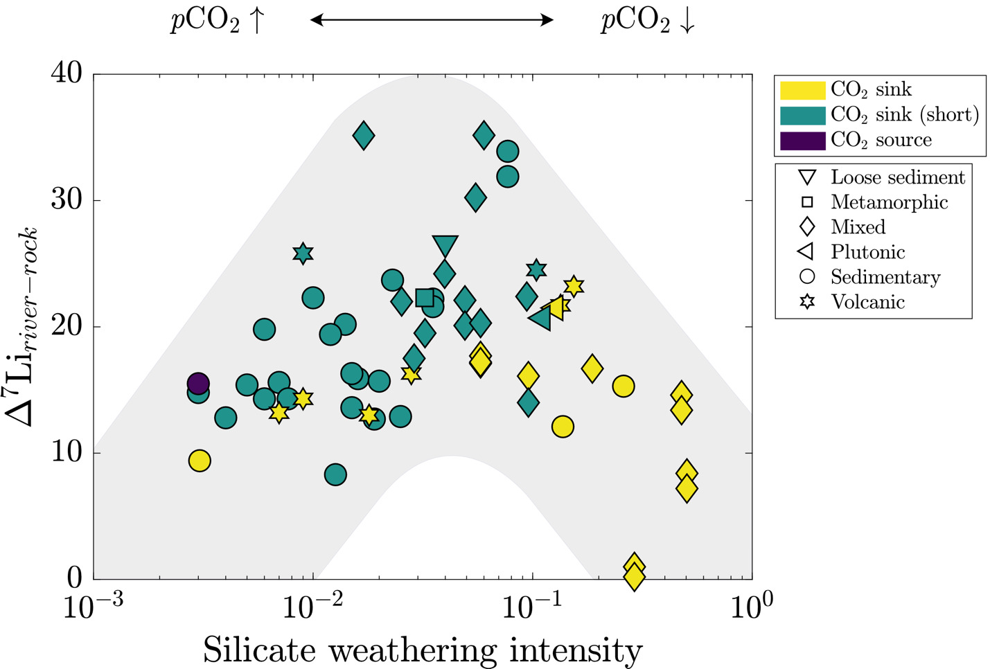
Ultimately, any attribution of the influence of clay formation on carbon cycle dynamics with Li isotopes must consider the supply and intrinsic dissolution rates of primary silicate minerals, rates of clay mineral formation, and their environmental associations. Previous Li isotope studies illustrate how this lens may be useful. During the Middle Eocene Climatic Optimum, where a positive Li isotope excursion is documented (Krause et al., 2023), the authors argue that the sluggish climate recovery results from enhanced cation uptake into clay minerals that diminishes the alkalinity supplied by silicate dissolution. The positive correlation between δ7Liriver values and clay alkalinity consumption (fig. 14D) makes clay cation retention a plausible explanation for the positive δ7Liseawater excursion during this event. Critically, the authors emphasize that enhanced cation uptake by clay was engendered by the existence of thick mantles of soil on continents prior to event onset, but it is unclear how these antecedent conditions favor enhanced clay formation and cation uptake since clay mineral formation is limited by the supply of fresh, silicate sediment. An alternative explanation could be that limited supply of fresh sediment, and thus low silicate dissolution and clay formation rates, inhibited a strong silicate weathering response. If true, the positive isotope excursion would be driven by an increase in the ratio of clay formation to primary silicate dissolution. This possible mechanism aligns with the interpretation of Pogge von Strandmann et al. (2013) where they attribute the recovery after an ocean anoxic event to the rapid weathering of freshly supplied flood basalts whose eruption initiated the event. This event is typified by a negative isotope excursion, which could be the result of a decrease in the ratio of clay formation to primary silicate dissolution.
5. CONCLUSIONS
Here we evaluated how river water Li isotope ratios relate to atmospheric CO2 changes during the chemical weathering of continental crust. We first compiled published δ7Liriver values and their associated solute concentrations and inverted these observations using the MEANDIR model to constrain solute sources and sinks. In comparing inversion results with the geologic and environmental attributes of their watersheds and equations of mass transfer during weathering, we evaluated the processes that drive first-order system behavior and weathering-induced carbon cycle effects. We found that δ7Liriver values positively correlated to the degree of alkalinity consumed by clay minerals for watersheds that are not dominated by volcanic rocks. Yet, these isotope ratios did not conform to a clear relationship with net weathering impacts on atmospheric CO2 due to complications related to a) the weathering of non-silicate minerals that alter the net ∆ALK/∆FIC from weathering and b) the different degrees of isotopic fractionation induced by the geologic and environmental drivers. We determined that river Li+/Na+ ratios and provide more compelling evidence for the controls of silicate weathering, modes of Li+ transfer across landscapes, and the net impact on atmospheric pCO2 due to weathering. The effects of bedrock geology and climate manifest clearly in predicted ∆ALK/∆FIC and Li uptake, where hot climates and cation-rich rocks tend to yield high ∆ALK/∆FIC and low and cold climates and cation-poor rocks tend to yield the opposite. Through our mass transfer calculations during crustal denudation, we find that the range of predicted carbon cycle effects and propensities for Li uptake via weathering can be conceptualized through the lens of mineral supply. Specifically, we assess that ∆ALK/∆FIC and are mutually driven by the intrinsic weatherability and mineralogical makeup of rocks and their rate of input through uplift, with climate playing an important but secondary role in the balance of weathering reactions and Li isotope fractionation. Uncertainty in model-predicted ∆ALK/∆FIC and δ7Liriver values principally arises from the balance of clay mineral formation rates, silicate dissolution rates, and the cationic charges they either supply to or uptake from solution, renewing the importance in further refining their rate constants and associated environmental drivers. These improvements are paramount in deducing the influence of clay mineral formation in the global carbon cycle and in interpretating Li isotopes records of past climate change.
ACKNOWLEDGMENTS
We thank D. O. Breecker and J. D. Barnes for detailed suggestions on earlier drafts of this manuscript and D. M. Rempe, J. P. L. Johnson, Z. T. Sickmann, and M. B. Cardenas for fruitful discussions and thoughtful input during this project. C. Meier shared data from the Pamirs, N. J. Planavsky shared data from Thailand, and S. Zhang assisted with implementing tools in ArcGIS, for which we are immensely grateful. This manuscript was improved by detailed comments from two anonymous authors and careful editorial handling by Associate Editor Kate Maher. This work was supported by NSF-EAR-2053056 (to E. J. Ramos), NSF-EAR-2204376 and the University of Chicago T.C. Chamberlin Fellowship (to P.C. Kemeny) and NSF-EAR-2017106 (to M.A. Torres).
SUPPLEMENTARY MATERIALS
MATLAB scripts and supplementary files for statistical analysis, MEANDIR inversions, modeling of silicate weathering, and figure generation can be found through Zenodo: https://doi.org/10.5281/zenodo.18406587
AUTHOR CONTRIBUTIONS
EJR designed the project and amassed the compilation. TNC conducted GIS analyses and determined watershed properties. EJR, PCK, and MAT designed the solute inversion, and EJR developed the mass balance model. All authors interpreted the results and wrote the manuscript.
CONFLICTS OF INTEREST
The authors declare no conflicts of interest.
Editor: C. Page Chamberlain, Associate Editor: Kate Maher