Balancing Redox Budgets: Mechanisms for Prolonging Anoxia During Major Carbon Burial Events

1. Introduction

Throughout Earth’s history, there have been many intervals of widespread marine anoxia, with the most well-studied having occurred during the Mesozoic. These events reflect major disturbances to global climate and environment that lasted for several hundreds of thousands of years or longer (Jenkyns, 2010). They indicate geologically short-term departures from typical steady-state oxygen content of the ocean-atmosphere system, which is often assumed to be a balancing of various known processes (Holland, 2002). Oceanic anoxic events (OAEs) are specifically defined as intervals of increased black shale deposition across multiple basins indicating widespread impact of geochemical changes to the ocean (Schlanger & Jenkyns, 1976). Therefore, one of the defining features of these events is the accumulation of organic-rich sediments across large portions of the ocean during these intervals (Jenkyns, 2010; Kemp et al., 2022; Owens et al., 2018; Schlanger & Jenkyns, 1976), as well as perturbations to various geochemical cycles, most notably those of carbon and sulfur, but also other redox-sensitive elements (Gill et al., 2011; Jenkyns, 2010; Owens et al., 2013, 2018; Them, Gill, Caruthers, et al., 2017). Many of these OAEs had important effects on life at the time, with some coinciding with major extinction intervals (Bond & Grasby, 2017; Jenkyns, 2010). Thus, studying these events can better relate Earth system processes to dynamic intervals of faunal turnover.

Constraining and quantifying the mechanisms that allow for these long-term intervals of enhanced organic matter burial and reducing marine conditions while maintaining near-modern atmospheric oxygen (O₂) contents has been greatly understudied. The primary cause for these events is often related to warming of the atmosphere and/or ocean system, leading to enhanced nutrient runoff from a heightened hydrologic cycle and weathering intensity (Gernon et al., 2024; Meyer & Kump, 2008). It has been proposed that the enhanced flux of nutrients increased the rates of marine primary productivity, whereby subsequent respiration and remineralization of that organic matter consumed dissolved O₂ (Gernon et al., 2024; Jenkyns, 2010; Poulton et al., 2015). This may be compounded by reduced thermohaline circulation and lower retention of dissolved gases in warmer waters (Meyer & Kump, 2008). The depletion of O₂ across these intervals causes aerobic respiration rates to decrease until the consumption of organic matter was less than the supply, at which point, sedimentary organic matter burial rates increased. Additional factors, such as remineralization rates of organic matter increasing with temperature, cause some inconsistencies that make this broad relationship non-linear.

1.1. Reduced carbon and sulfur burial effects on oxygen

With respect to O₂ production, it has been shown through decades of work that the most important reduced compounds buried are species of carbon and sulfur (e.g., organic carbon, organic sulfur, and pyrite) (Berner, 2006; Berner & Canfield, 1989; Garrels & Lerman, 1981). The production and burial of these compounds require the release of O₂ as the product in the reaction (table 1). Since some organic carbon and pyrite sulfur are buried and sequestered from the system, they become unavailable for O₂ consumption, causing O₂ content of the ocean-atmosphere system to increase. Modeling efforts, such as GEOCARBSULF, have quantified the burial of carbon and sulfur as a means to document the long-term O₂ budget of the Earth’s surface (Berner, 1991, 2006, 2009; Berner & Canfield, 1989; Berner & Kothavala, 2001). The GEOCARBSULF model (Berner, 2006) and prior GEOCARB model (Berner & Canfield, 1989) utilize the presence of organic carbon-rich rocks in the sedimentary record and the burial of pyrite, both interpreted through isotope work, to determine the amount of O₂ production from burial of reduced species entering the atmosphere through the Phanerozoic using bins of several million years (i.e., longer than short-term OAEs). These calculated O₂ contents are modulated by many different mechanisms, but are mainly calculated using global marine carbon and sulfur isotope compositions to estimate the burial of organic carbon and pyrite sulfur (Berner, 2006; Berner & Canfield, 1989; Berner & Kothavala, 2001).

Similar studies have focused on the potential of carbon and sulfur burial to increase O₂ across the Great Oxidation Event and Lomagundi carbon isotope excursion (CIE), the Neoproterozoic Oxygenation Event and Shuram CIE, and the Cambrian rise in O₂ (Bristow & Kennedy, 2008; Eguchi et al., 2020; Miyazaki et al., 2018; Saltzman et al., 2011). Other models utilize similar concepts with other variables, evidence and datasets, such as the COPSE model (Bergman et al., 2004). These studies have suggested that the burial of vast quantities of reduced carbon and sulfur induced O₂ production and global oxygenation, yet Phanerozoic anoxic events also buried copious amounts of these compounds but instead are associated with deoxygenation. Thus, there is disconnect for these shorter timescale events. Notably, the burial of carbon and sulfur has also been linked to changes in phosphorus cycling due to this element being a major bioessential nutrient (Van Cappellen & Ingall, 1994), and such changes have been modeled to show notable fluctuations corresponding with important carbon cycle perturbations that relate to these increases in O₂ (Bergman et al., 2004; Reershemius & Planavsky, 2021; Reinhard & Planavsky, 2022).

This quantitative approximation through modeling is a similar process to what is implemented across Mesozoic OAEs, where carbon and sulfur geochemistry is utilized to estimate the burial of their respective reduced species (Gill et al., 2011; Jenkyns, 2010; Kemp et al., 2022; Owens et al., 2013, 2018; Ruebsam & Schwark, 2024; Them et al., 2022), yet the O₂ production that such burial would cause are often under-discussed in favor of just quantifying this burial solely as an effect of widespread anoxia during such multi-millennial events due to proxy sensitivity (e.g., Dickson et al., 2017; Gill et al., 2011; Owens et al., 2013, 2018; Them, Gill, Caruthers, et al., 2017). Therefore, the burial of reduced chemical species should be investigated as a negative feedback mechanism that should cause O₂ production during the development of an OAE. This re-oxygenation feedback should occur on the tens of thousands of year timescale such that OAEs should be self-limiting in duration (Reershemius & Planavsky, 2021).

There are a variety of other phenomena that could extend the duration of OAEs, such as reactivity rates of organic carbon and pyrite sulfur formation, changes to ocean mixing times, stratification of seawater, or localized development of anoxia, both temporally and spatially. All of these would increase the duration of OAEs from durations of typical ocean-atmosphere circulation (~1,000 to 6,000 years), but not to the order magnitudes suggested by the geologic record. If other processes slow the rate of O₂ release from the burial of reduced species, it could limit this reoxygenation until after the OAE due to atmospheric oxygen response time being longer than the event itself. Subsequently, the excess O₂ could result in measurable and resolvable changes in various ocean-atmospheric processes and biologic impacts following the event. There is no evidence from the sedimentary record to support this; instead, evidence for concurrent increases in wildfire across the Toarcian OAE and Cretaceous OAE-2 suggest that O₂ may have been higher in the atmosphere during but not following the events (S. J. Baker et al., 2017; Boudinot & Sepúlveda, 2020). Additionally, other evidence suggests low oxygen conditions in marine bottom waters persisted long after these events rather than oxygenation (Ostrander et al., 2017; Them et al., 2018). Therefore, the temporal extent of these events and lack of oxygen accumulation post-event (Bond & Grasby, 2017; Jenkyns, 2010) indicates additional processes must have occurred to sustain deoxygenation.

1.2. Mechanisms to reduce excess oxygen

The emplacement of large igneous provinces (LIPs) often coincide with OAEs and provide causal mechanisms for these global-scale marine deoxygenation intervals (Bond & Grasby, 2017; Green et al., 2022; Jiang et al., 2023; Kasbohm et al., 2021). LIPs supply a significant flux of mantle-derived carbon, primarily CO₂ (Bond & Grasby, 2017; Burgess et al., 2015; Fendley et al., 2024; Kasbohm et al., 2021), to the atmosphere, causing the climatic shifts likely needed to induce these events. This is often compounded by thermogenic carbon released from contact metamorphism of sedimentary rocks by the igneous intrusions (Chang et al., 2022; Flögel et al., 2011; Heimdal et al., 2021; Them, Gill, Caruthers, et al., 2017) or other feedbacks (e.g., wildfires, methane release from clathrate or wetlands) that also introduce carbon into the atmosphere from other sources (S. J. Baker et al., 2017; Boudinot & Sepúlveda, 2020; Huang et al., 2024; Them, Gill, Caruthers, et al., 2017). Additionally, other LIP-sourced materials, such as SO₂, aerosols, and particulates, may also induce major climatic changes, though these primarily induce short-term cooling (Bond & Grasby, 2017; Kasbohm et al., 2021).

This volatile-induced climate change has been a primary focus for research on the OAE-LIP relationship, but these volcanic provinces also likely introduced a variety of other reduced materials, such as iron (Fe²⁺), manganese (Mn²⁺), hydrogen sulfide (H₂S), hydrogen (H₂), methane (CH₄), and ammonia (NH₃) to the exogenic Earth during their emplacement (Edmonds et al., 2022; Sinton & Duncan, 1997). Such reducing species would react with available O₂, thereby removing it from the ocean-atmosphere system (table 1). There is additional evidence reducing volcanic emissions help counterbalance global redox changes from the formation of organic matter to some degree in the modern (Holland, 2002). However, limits on our knowledge of the size and timing of eruptive activity as well as volatile composition, make it difficult to quantify the flux of reductants that LIPs could have been introduced to the system.

While size and timing of LIPs remain major focus of study, (Jiang et al., 2023; Kasbohm et al., 2021), their volatile chemistry remains comparatively understudied (Capriolo et al., 2021). Though not perfectly comparable to the subaerial LIPs that are the focus of this study, volatile flux estimates from modern hydrothermal systems at seafloor spreading centers were utilized here to approximate those from LIPs (Kasbohm et al., 2021; Mason et al., 2021). Other modern systems, namely mantle-plume-derived systems, suggested to be the most appropriate modern analog to LIPs, were also explored as LIP volatile analogs (Ilyinskaya et al., 2021; Jones et al., 2016; Mason et al., 2021; Self et al., 2008). However, differences in their volume and the areal extent of emissions compared to LIPs (most of these measurements are limited to singular vents), lack of data for some reduced compounds, and resulting flux estimations that ranged several orders of magnitude meant flux estimates from these systems were not utilized in this study (supplemental discussion). Further, work on emission from mantle-plume-derived systems (Campbell, 2005), suggest they are more similar to mid-oceanic ridge systems in terms of the redox potential of their emissions when compared to less reduced volcanic arcs systems (Holland, 2002). Overall, this indicates the assumption to utilize modern hydrothermal fluxes as analogs for LIP emissions is a reasonable approach.

That being said, there are certainly differences between mid-ocean ridge and subaerial LIPs systems (e.g., the infiltration of fluids into continental versus marine rocks and sediments) that may induce additional chemical changes that we do not account for here (Burgess et al., 2017; Green et al., 2022). However, even with the potential large uncertainties in estimating LIP reductant loads, the timing of the main phase(s) of LIP activity is often still well-correlated to time-equivalent OAEs, and many of their emplacements last as long as, if not longer than, their associated OAE (Bond & Grasby, 2017; Jiang et al., 2023; Kasbohm et al., 2021). Therefore, the LIPs likely still released significant amounts of reduced compounds over the duration of these OAEs and must be considered when quantifying their global redox budgets.

An additional source of O₂ consumption is from oxidative weathering and is considered in both the GEOCARB and GEOCARBSULF models (Berner, 2001, 2006; Berner & Canfield, 1989; Berner & Kothavala, 2001). There is evidence for increased chemical weathering across many OAEs and is likely related to higher global temperatures and an enhanced hydrologic cycle (Frijia & Parente, 2008; Kemp et al., 2020; McArthur et al., 2000; Percival et al., 2016; Pogge von Strandmann et al., 2013; Them, Gill, Selby, et al., 2017). Though chemical silicate weathering intensities do not directly relate to oxidative weathering, enhancement in silicate weathering is likely to correspond to increased oxidative weathering nonlinearly due to increases in physical weathering and enhanced hydrologic cycle effectively exposing fresh material to the oxygenated atmosphere (Berner, 2006; Berner & Kothavala, 2001; Daines et al., 2017; Gabet & Mudd, 2009). However, this nonlinear aspect is further compounded by the difference in oxidative weathering rate of reduced species, where sulfide minerals (e.g., pyrite) tend to oxidize more rapidly than organic matter during oxidative weathering (Littke et al., 1991; Petsch et al., 2000). In addition, there is a greater likelihood that younger, more liable reduced compounds are more rapidly oxidized, compared to longer-buried, more recalcitrant ones (Berner, 2006). This indicates that the age of exposed material is relevant but has limited applicability on the temporal scales that are the focus of this study (maximum of 10 million years) compared to long-term O₂ budget studies that involve more tectonic processes, which have bins around 10 million years (Berner, 2006, 2009). Thus, the relationship between silicate weathering intensity and oxidative weathering intensity is hard to quantify due to nonlinear interactions. However, a simplified relationship coupled with large and varied sensitivity tests in the model can give rough ranges for the effect of oxidative weathering on excess O₂ contents similar to approximations provided by the GEOCARBSULF model (Berner & Kothavala, 2001).

To analyze the net change in O₂ and potential chemical relationship between LIPs, oxidative weathering, and the redox evolution across OAEs, we focused on two of the most heavily studied OAEs, Oceanic Anoxic Event 2 (OAE-2, ~94 Ma) in the Cretaceous (Cenomanian-Turonian stage transition) and the Toarcian Oceanic Anoxic Event (T-OAE, ~184 Ma) in the Early Jurassic (post-Pliensbachian-Toarcian boundary). Both events have been primarily defined in recent work by their major associated CIEs as a chemostratigraphic markers (fig. 1A–B) and intervals of the widespread deposition of organic-rich sediments (Beerling & Brentnall, 2007; Bond & Grasby, 2017; Boulila et al., 2014; Dickson et al., 2017; Erbacher et al., 2005; Gill et al., 2011; Jenkyns, 1988; Y.-X. Li et al., 2017; Owens et al., 2013; Them, Gill, Caruthers, et al., 2017), but also supplementarily dated with biostratigraphic markers (Boulila et al., 2014; Corbett et al., 2014; Elder, 1989; Morten & Twitchett, 2009). Mass balance and forward box models were used to determine the O₂ produced via organic carbon and pyrite sulfur burial compared to its consumption from the reductants released from the respective LIPs and oxidative weathering. Both O₂ consumption mechanisms, LIP reductants and oxidative weathering, were considered in isolation to determine their net effect on oceanic O₂. Previous models of carbonate carbon isotopic variation across OAE-2 (Owens et al., 2013) and estimates of total organic carbon burial for the T-OAE (Them et al., 2022) along with carbonate-associated sulfate (CAS) sulfur isotopes for both events (Gill et al., 2011; Owens et al., 2013) were used to determine the organic carbon and pyrite sulfur buried, respectively (fig. 1C–D). The combination of O₂ production and O₂ consumption models presented here are a broad attempt to better constrain the O₂ budgets during OAEs beyond previous work with its limitations and assumptions discussed below.

Figure 1.Idealized carbon isotopes and previously modeled carbon and sulfur isotopes of OAE-2 (A, C) and the T-OAE (B, D). (A) Idealized carbonate carbon isotopes of OAE-2 (Dickson et al., 2017; Erbacher et al., 2005), divided up into pre-CIE (K1), syn-positive CIE (K2), and post-CIE (K3). (B) Idealized carbonate carbon isotopes of the T-OAE (Them et al., 2022), divided up into Pliensbachian (J1), pre-CIE (J2), syn-negative CIE (J3), post-CIE (J4), and return to baseline (J5). (C) Modeled carbon and sulfur isotopic excursions of OAE-2 from previous work (Owens et al., 2013, 2018). (D) Modeled sulfur isotopic excursion from previous work on the T-OAE (Gill et al., 2011) and new modeled carbon isotopic excursion based on carbon burial data implied by Mo/TOC for the T-OAE (Them et al., 2022), excluding sources of ¹³C-depleted carbon that would induce the observed negative CIE. Grey boxes represent approximate timing of main phase LIP activity for the respective OAE. Cenom. = Cenomanian, Pliens. = Pliensbachian.

1.3. Oceanic Anoxic Event 2

The record of the OAE-2 has been identified as the appearance of organic-rich sediments in various Upper Cretaceous sedimentary successions globally (Boudinot & Sepúlveda, 2020; Eldrett et al., 2015; Erbacher et al., 2005; Jenkyns, 2010; Meyers et al., 2012; Owens et al., 2018; Raven et al., 2019). This event also has a distinct positive CIE and positive sulfur isotope excursion associated with it (Dickson et al., 2017; Eldrett et al., 2015; Erbacher et al., 2005; Owens et al., 2013). These two features most likely indicate the enhanced burial of organic carbon and pyrite sulfur, respectively, on a globally relevant scale (Owens et al., 2013; Raven et al., 2019). The positive CIE is often used to define the duration event itself, and the interval containing it is associated with indicators of relatively warmer global temperatures (Bond & Grasby, 2017; Erbacher et al., 2005; Owens et al., 2013, 2018), increased silicate weathering (Frijia & Parente, 2008; Pogge von Strandmann et al., 2013; Poulton et al., 2015), enhanced nutrient runoff from the continents (Y.-X. Li et al., 2022; Poulton et al., 2015), expansion of seafloor anoxia (Clarkson et al., 2018; S. Li et al., 2023; Montoya-Pino et al., 2010; Ostrander et al., 2017), and elevated rates of extinction, albeit only marginally greater than background rates (Bond & Grasby, 2017; Coccioni & Galeotti, 2003; Elder, 1989). The wealth of available geochemical information has been the subject of numerous investigations, especially the carbon and sulfur cycles across the event, making it an ideal interval of study to determine the potential increases in O₂ production due to the burial of reduced species.

One of the difficult challenges for understanding the drivers of OAE-2 is the number and variety of LIPs that have been invoked with this event. This is primarily due to poor age constraints for the associated LIPs. The Ontong Java LIP, Kerguelen LIP, Madagascar LIP, Caribbean Plateau LIP, and High Arctic LIP (HALIP) have all been suggested to coincide with OAE-2 (Jiang et al., 2023; Kasbohm et al., 2021; Maher, 2001; Sinton & Duncan, 1997). Nevertheless, many studies suggest that the Caribbean Plateau LIP (97 to 80 Ma), located in the modern-day Caribbean Sea, is the primary driver due to the radiometric dates of this submarine LIP closely aligning with the timing of OAE-2 and its large spatial extent (Jiang et al., 2023; Kasbohm et al., 2021). HALIP (93 to 89 Ma), a partially subaerial LIP located primarily in the Arctic Ocean and on several surrounding landmasses, also has a coeval date with OAE-2 (Jiang et al., 2023; Maher, 2001). Its major eruptive interval approximately spans 2 million years (Myr), and HALIP currently covers an area of approximately 200,000 km² (Kasbohm et al., 2021; Maher, 2001). Better spatial constraints and radiometric dating of this LIP (Jiang et al., 2023; Maher, 2001), as well as evidence of weathering of atmospherically exposed basaltic material (Pogge von Strandmann et al., 2013; Sullivan et al., 2020), make HALIP potentially a more suitable target for this study’s models. Additionally, other continental LIPs are better associated with known global environmental perturbations throughout Earth History while few marine LIPs are (Green et al., 2022). This suggests that HALIP may have also been a greater contributor to this event.

Due to the limited dates on the LIP material, various scenarios of LIP activity were considered, including one based on the marine osmium records (Sullivan et al., 2020). This latter option includes three phases of volcanism that may have occurred during the early stages of OAE-2 (Y.-X. Li et al., 2022; Sullivan et al., 2020). Still, there is a lack of direct correlation between this proxy evidence of LIP activity and precise radiometric dating of HALIP volcanic deposits. The osmium isotope record also suggests significantly shorter volcanic activity than most estimates for the duration of HALIP and/or the other LIPs that have been associated with OAE-2 (Jiang et al., 2023; Kasbohm et al., 2021), and is therefore likely a conservative estimate for LIP activity. Given this uncertainty, various other modeling scenarios for LIP eruptions were included in our scenarios for OAE-2.

Various proxies have been applied to the record of OAE-2 to constrain chemical silicate weathering rates and intensities. Osmium, lithium, and strontium isotopes proxies have all been applied to this OAE to approximate changes in silicate weathering and indicate a major increase in chemical weathering during the event (Frijia & Parente, 2008; Pogge von Strandmann et al., 2013; Poulton et al., 2015; Sullivan et al., 2020). The increases in silicate weathering have been linked to increased temperatures and hydrologic cycle activity (Gernon et al., 2024; Pogge von Strandmann et al., 2013; Poulton et al., 2015). Therefore, the estimated, model-derived 2 to 3 times increase in silicate weathering intensities across 200 thousand years (kyr) during OAE-2, which can provide an overall weathering rate increase for this interval, was utilized and likely had an impact on the oxidative weathering that could be incorporated into the model (Pogge von Strandmann et al., 2013).

1.4. Toarcian Oceanic Anoxic Event

The Early Jurassic T-OAE has also been identified from widespread organic matter-rich deposition at localities around the world (Cohen et al., 2004; Jenkyns, 1988, 2010; Kemp et al., 2022; Pálfy & Smith, 2000; Ruebsam et al., 2022; Ruebsam & Schwark, 2024; Them, Gill, Caruthers, et al., 2017). There is a noted CIE associated with this event, but it is a major negative excursion (~4–6‰) that likely represents greater input of isotopically light carbon to the ocean-atmosphere system (Beerling & Brentnall, 2007; Bond & Grasby, 2017; Fendley et al., 2024; Gambacorta et al., 2024; Heimdal et al., 2021; Hesselbo et al., 2007; Jenkyns, 2010; Kemp et al., 2020; Ruebsam & Schwark, 2024; Them, Gill, Caruthers, et al., 2017). However, this negative CIE does not imply a lack of enhanced organic carbon burial during this event as evidenced by the occurrence of Toarcian organic-rich strata (Gambacorta et al., 2024; Kemp et al., 2022; Ruebsam et al., 2022; Ruebsam & Schwark, 2024). Further, a longer-term (3–4 Myr) positive CIE (~1–2‰) is found around the T-OAE, that is interrupted by the short-lived prominent negative CIE (Jenkyns, 2010; Them, Gill, Caruthers, et al., 2017) that has been interpreted to indicate enhanced carbon burial surrounding the T-OAE (Gambacorta et al., 2024; Jenkyns, 2010; Ruebsam & Schwark, 2024; Them et al., 2022; Them, Gill, Caruthers, et al., 2017). It, therefore, has been suggested that the positive carbon isotopic shift was transiently overwhelmed by the input of light carbon to induce a negative CIE (S. J. Baker et al., 2017; Ruebsam & Schwark, 2024; Them, Gill, Caruthers, et al., 2017).

Estimating organic carbon burial rates from this carbon isotope record is made complicated by the combined signals of the long-term positive and short-term negative CIEs. There has been much work focused on constraining the potential sources of ¹³C-depleted carbon to the Earth system to account for this major negative CIE (S. J. Baker et al., 2017; Beerling & Brentnall, 2007; Huang et al., 2024; Kemp et al., 2020; Them, Gill, Caruthers, et al., 2017), but less emphasis on determining carbon burial and the budgets of the ocean-atmosphere O₂. Other methods have to be employed to estimate organic carbon burial across the T-OAE either through globally mapping organic carbon contents of lithologies across this interval (Kemp et al., 2022; Ruebsam & Schwark, 2024) or comparing organic carbon content to other chemical proxies not affected by this pool of isotopically light carbon (Them et al., 2022). This latter method was employed due to the limited global mapping available (only around the Tethys) to provide sufficient model parameters (Kemp et al., 2022; Them et al., 2022).

Beyond this complication regarding the carbon isotope records, the T-OAE has many other well-constrained parameters that are useful for this study. There is a well-documented CAS sulfur isotope excursion that effectively estimates global pyrite burial (Gill et al., 2011). This interval, like OAE-2, is associated with rising global temperatures (Nordt et al., 2022), increased silicate weathering intensity (McArthur et al., 2000; Percival et al., 2015; Them, Gill, Selby, et al., 2017), enhanced nutrient runoff from the continents (Beerling & Brentnall, 2007; Kemp et al., 2020; Them, Gill, Selby, et al., 2017), expansion of seafloor anoxia (Gill et al., 2011; Them et al., 2018), and greatly elevated rates of extinction (Morten & Twitchett, 2009; Wignall et al., 2006, 2010), all of which are generally greater than equivalent changes for OAE-2.

What is well-constrained for the T-OAE is its strong temporal coincidence with the Karoo-Ferrar (K-F) LIP (185 to 181 Ma) (Burgess et al., 2015; Greber et al., 2020; Jiang et al., 2023; Kasbohm et al., 2021). This is one of the largest continental LIPs of the Phanerozoic (Jiang et al., 2023; Kasbohm et al., 2021), with a total surface area of 920,000 km², separated into the Karoo province of Southern Africa and Ferrar province of Antarctica (Burgess et al., 2015; Kasbohm et al., 2021). Volcanic activity primarily spanned 4.5 Myr, though the major phases occurred over a smaller 300-kyr interval (Burgess et al., 2015; Greber et al., 2020).

In regard to weathering proxy records, there are less Toarcian records compared to OAE-2 and the primary proxy that has been applied in this regard is sedimentary osmium isotopes (Cohen et al., 2004; Kemp et al., 2020; Percival et al., 2016; Them, Gill, Selby, et al., 2017). There are potentially longer-term changes in weathering flux indicated in seawater strontium isotope record (McArthur et al., 2000), though these data do not aid with quantifying this flux during the shorter interval of the T-OAE due to strontium’s longer residence time in the ocean. The osmium isotope data suggest a short-term (100 to 200 kyr) increase in silicate weathering intensity, 3 to 6 times greater than the modern intensities (Kemp et al., 2020), which again can be converted to average rate increase based on the known intensity and duration.

2. Methods

2.1. Calculations for LIP reductant composition

To determine LIP reductant composition, data from modern hydrothermal activity of mid-oceanic ridges was utilized as an approximation. These were calculated by compiling the concentration of volatiles (in μmol/kg) from various hydrothermal systems (supplemental table 1). The volatiles that were included were Fe²⁺, Mn²⁺, H₂S, H₂, CH₄, and NH₃ (Charlou et al., 2000; Evans et al., 1988; Ishibashi et al., 2015; James et al., 2014; Ji et al., 2017; McDermott et al., 2018; Reeves et al., 2011; Seyfried et al., 2015; Von Damm, 1990) as previously utilized by earlier attempts to quantify O₂ reduction during OAEs (Sinton & Duncan, 1997). Due to the high variability in measured concentrations and various compounds having only limited data, the median concentrations were utilized for each compound. These were each then multiplied by the total global annual flux of hydrothermal material, an average of 7.2 × 10¹² kg/yr (Nielsen et al., 2006), to result in a global flux for each compound (in mol/yr). Last, this was divided by the total global surface area of hydrothermal activity, 1.2 × 10¹² km² (E. T. Baker & German, 2004; Nielsen et al., 2006; Von Damm, 1990), to reach a reasonable approximation for the flux of each of these reductants per unit area. A similar methodology was attempted using island plume activity, mainly from Hawaii, but limitations in data and calculations proved this to be less useful (supplemental table 2). Due to the uncertainties of the comparability of LIP volatile fluxes to those of seafloor hydrothermal systems, this variable is modulated between half to double modern hydrothermal rates.

2.2. Forward Box Models for O₂ production

Forward geochemical box models were utilized for determination of net O₂. These models assumed steady state of the O₂ budget prior to the event. Thus, the results from most of the following equations and models are represented as changes from this steady state scenario rather than the actual abundances that may have existed in the ocean-atmosphere system, but these were also calculated through subtracting from the initial steady state values. For the production of O₂ from organic carbon and pyrite sulfur burial, box models of the carbon and sulfur cycles for OAE-2 (Owens et al., 2013) and the sulfur cycle for the T-OAE (Gill et al., 2011) were recreated (fig. 1). These used a time-dependent equation for the isotopic composition of the marine carbonate and sulfate reservoirs to reconstruct the marine isotope curves of these proxies. The following equation is for the time-dependent changes in marine carbonate carbon isotopes (a similar framework was applied to the sulfur cycle):

$$\frac{d\delta_{carb}}{dt} = \ \frac{\sum_{\mathstrut}^{\mathstrut}{F_{in}\ (\delta_{in}\ - \ \delta_{sea})}\ - \ \sum_{\mathstrut}^{\mathstrut}{F_{out}\Delta_{out}}}{M_{0}},\tag{1}$$

where δ_carb is the isotopic composition of the recorded values in carbonate (for the sulfur cycle this would be δ_sulf); δ_sea is the isotopic composition of the ocean at the time and is equivalent to δ_carb or δ_sulf; F_in are the input fluxes to the ocean of the respective isotopic system being modeled in moles per year with an isotopic composition of δ_in; F_out are the output fluxes from the ocean of the respective isotopic system being modeled in moles per year with a offset from seawater isotopic values of Δ_out, and M₀ is the initial amount of the respective element in the ocean reservoir in moles. For the carbon cycle, the only input is weathering, with the outputs being carbonate formation and organic carbon burial. See the later discussion for lack of including inputs of volcanogenic and thermogenic carbon. For sulfur, the inputs were weathering and hydrothermal fluxes and the outputs of sulfate and pyrite burial. For specific details on the initial parameters utilized and sensitivity tests to approximate isotopic curves found in the geologic record, see previous cited studies (Gill et al., 2011; Owens et al., 2013). For the purposes of this project, only the carbon burial rates and pyrite sulfur burial rates for the sensitivity tests thought to be most representative were utilized in our study for O₂ production during OAEs.

The organic carbon burial rates for the T-OAE utilized other studies based on molybdenum (Mo) to total organic carbon (TOC) ratios (Them et al., 2022) and a smaller estimate based primarily on an accounting of preserved organic-matter deposits formed during the event (Kemp et al., 2022). This new model attempts to recreate the T-OAE positive CIE based on organic carbon burial and not the major negative CIE likely caused by the large input of ¹³C-depleted carbon from volcanism and other sources (Ruebsam & Schwark, 2024; Them, Gill, Caruthers, et al., 2017) using equation (1), as illustrated in figure 1B. Due to poorer constraints on organic carbon burial with the method utilized, the full range of estimated burial values from Them et al. (2022) and Kemp et al. (2022) were utilized for the model across the time interval studied instead of a single reasonable estimate for carbon burial rate as for OAE-2.

Stoichiometric calculations (table 1) were used to determine the amount of O₂ produced due to the burial of organic carbon and pyrite (table 2). This utilized the equation:

$$\begin{align} O_{P}(t) &= 1*\left( F_{org}(t) - F_{org}(0) \right) \\&\quad+ 3.5*(F_{py}(t) - F_{py}(0)). \end{align} \tag{2}$$

where O_P is excess O₂ produced in moles; F_org is organic carbon burial in moles per year; F_org(0) is initial organic carbon burial rate; F_py is pyrite burial in moles per year; and F_py(0) is initial pyrite burial rate. The initial values, representative of baseline conditions prior to each event, were removed so that only excess O₂ production could be calculated rather than total O₂ production.

2.3. Forward Box Models for O₂ consumption

Additions to the forward geochemical box models were used to approximate the reducing components of the related LIPs, using the HALIP for OAE-2 (Kasbohm et al., 2021; Maher, 2001; Sinton & Duncan, 1997) and K-F LIP for the T-OAE (Burgess et al., 2015; Greber et al., 2020; Kasbohm et al., 2021). As there are relatively few estimates of the overall reductant load from these LIPs (Kasbohm et al., 2021; Sinton & Duncan, 1997), the reductant output of modern mid-oceanic ridge hydrothermal vent activity per surface area was utilized (supplemental table 1). Most recent estimates for duration and geographic extent of the LIPs were utilized for the modeled excursion of reductant material (Burgess et al., 2015; Kasbohm et al., 2021; Maher, 2001; Sinton & Duncan, 1997). These model parameters are in table 2. Variations on the extent of reductant output, aerial extent, duration, possible pulses of volcanism, weathering rates, and relation between silicate and oxidative weathering were modeled (table 3). Again, stoichiometric conversions were used to determine the amount of O₂ consumed due to the release of these reduced compounds (table 1). This results in the equation:

$$\begin{align} &O_{CLIP}(t) \\&\quad= A_{LIP}(t)*S_{LIP}(t)\\&\qquad*(0.25F_{Fe} + 0.5F_{Mn} + 1F_{H2S} \\&\qquad \quad + 2F_{CH4} + 0.5F_{H2} + 1.25F_{NH3}), \end{align} \tag{3}$$

where O_CLIP is excess O₂ consumed by LIP reductants, A_LIP is the unitless scaling factor of LIP activity compared to modern hydrothermal activity (with 1 equivalent to modern hydrothermal reductant load per unit area per time), S_LIP is the surface area of active LIP in km², and F_x represents the fluxes of various compounds derived from volcanic and hydrothermal activity in moles per km² per year. For the surface area of the LIPs, HALIP was assumed to be 200,000 km² for OAE-2 (Kasbohm et al., 2021; Maher, 2001) and the K-F LIP was modulated between 350,000 km² and 920,000 km² based on the specifically active province and the timing of active phases (Burgess et al., 2015; Greber et al., 2020; Jiang et al., 2023; Kasbohm et al., 2021). If the values of fluxes for modern hydrothermal activity (supplemental table 1) are included directly into equation (3), it can be simplified to create:

$$\begin{align} O_{CLIP}(t) &= {\left( 6.24\ \times 10^{12}mol\ {Myr}^{- 1}\ {km}^{- 2} \right)}\\ &\quad*A_{LIP}(t)*S_{LIP}(t). \end{align}\tag{4}$$

As thermogenic CH₄ has often been invoked as a major contributor to the climatic shifts at these times and is related during the emplacement of LIPs (S. J. Baker et al., 2017; Chang et al., 2022; Fendley et al., 2024; Heimdal et al., 2021), this parameter was varied for these events, increasing up to 3.00 × 10⁵ mol/yr/km² to account for potentially greater variability, and this change will slightly affect the flux term in equation (4).

To estimate oxidative weathering rates, the relationship from GEOCARB and GEOCARBSULF was utilized (Berner & Kothavala, 2001). It quantifies the relationship between silicate weathering rates and erosion rates as:

$$R_{w} = k*{(R_{e})}^{2/3},\tag{5}$$

where R_w is the weathering rate (specifically, silicate weathering), k is a constant, and R_e is the erosion rate (Berner & Kothavala, 2001). Assuming changes in erosional rates are directly related to oxidative weathering rates and that removing the k constant will not change the proportional difference between oxidative weathering and erosion when the modern rates of both are known, a new equation was created:

$$F_{ow}(t) = (F_{owc} + F_{ows}){{*R}_{cw}(t)}^{r},\tag{6}$$

where F_ow is the effective oxidative weathering rate, F_owc and F_ows are the modern oxidative weathering rates of carbon and sulfur, respectively, R_cw is the effective chemical silicate weathering rate compared to modern (assuming current relative weathering rate is 1), and r is the weathering relationship between silicate weathering and oxidative weathering. The r variable is initially set to 1.5 as prescribed by the GEOCARB and GEOCARBSULF models (Berner, 2006; Berner & Kothavala, 2001) since this relationship is inverted from equation (5) and is changed to a variable in order to explore this poorly constrained relationship. This variable is intended to cover the variety of potential uncertainties when comparing oxidative weathering to silicate weathering, including differences in weathering intensity of different compounds of different ages as well as other factors that lead to non-linear interactions between the two weathering types.

Since the modern oxidative weathering rates of organic carbon and pyrite sulfur have been estimated, 2.33 × 10¹² and 0.83 × 10¹² mol/yr, respectively (Burke et al., 2018; Daines et al., 2017), these can be substituted into the equation when combined with the oxygen consumption stoichiometry of organic carbon and pyrite sulfur (table 1). When introduced to the oxygen budget, the equation is:

$$\begin{align} O_{Cweath}(t) &= \left( 5.24\ \times 10^{18}mol\ {myr}^{- 1} \right)\\&\quad*{{(R}_{cw}(t)}^{r} - 1), \end{align}\tag{7}$$

where O_Cweath is excess O₂ consumed by oxidative weathering and the initial value is subtracted to determine only excess oxygen consumption from oxidative weathering.

Both the LIP reductant and oxidative weathering were separately modeled and then combined to show changes in O₂ over time (figs. 2–6). This involved combining the outputs of equations (2) with equation (3) and/or (7), creating:

$$O_{N}(t) = O_{P}(t) - \ O_{C}(t), \tag{8}$$

where O_N is net O₂. O_C was set to either O_CLIP (eq 3) or O_Cweath (eq 7). Some scenarios were run with these together as a combined O₂ consumption (O_C = O_CLIP + O_Cweath). Net O₂ contents of all runs are displayed in supplemental tables 4 and 5. These values were further compared to determine the degree of O₂ removal as a percentage of the produced O₂:

$$\% O_{2}\ consumed = \frac{O_{C}(t)}{O_{P}(t)},\tag{9}$$

and these results are presented (supplemental discussion and supplemental figs. 2–6).

Each model run was conducted over a 10-million-year span to include the buildup and decline of the CIE, LIP activity, weathering rates, and all other pertinent phenomena related to these events. Iterations in inputs occurred every 5,000 years, with outputs every 1,000 years. Starting parameters (table 2) were incorporated across all iterations, while various other parameters were tested (table 3) in accordance with the specifics dependent on the OAE’s available data and assumptions (supplemental tables 4–5).

Figure 2.Net O₂ production based on buried organic carbon and pyrite sulfur compared to LIP reductant input for OAE-2 across various sensitivity tests. (A) Modeled continuous volcanism across 2 Myr starting at the onset of OAE-2 (K2) modulating the total reductant output. (B) Modeled impact of two pulses of volcanism, each lasting 500 kyr. (C) Modeled impact of two pulses of volcanism, each lasting 700 kyr. (D) Modeled impact of four pulses of volcanism, each lasting 200 kyr. (E) Modeled impact of three pulses of volcanism based on the timing of osmium excursions (Y.-X. Li et al., 2022; Sullivan et al., 2020). (F) Modeled impact of increased CH₄ release based on thermogenic carbon estimates (Chang et al., 2022) compared to the continuous run with 1.0× LIP activity (A), though the difference between this run and the 0.5× additional CH₄ makes them indistinguishable in figure. The 0.0× LIP model runs show the total O₂ produced via burial of reduced carbon and sulfur without additional reductants from LIP activity.

Figure 3.Net O₂ production based on buried organic carbon and pyrite sulfur compared to oxidative weathering for OAE-2 across various sensitivity tests. (A) Modeled increases in weathering (Pogge von Strandmann et al., 2013) at the onset of OAE-2 (K2). (B) Modeled impact of changing the ratio utilized for r (see Methods) from a baseline of 1.5 with the average weathering rate of 2.5× (Berner & Kothavala, 2001). The 0.0× weathering model runs show the total O₂ produced via burial of reduced carbon and sulfur without additional oxidative weathering.

Figure 4.Net O₂ production based on buried organic carbon and pyrite sulfur compared to LIP reductant input for the T-OAE across various sensitivity tests for LIP activity. All panels use different amounts of organic carbon burial based on previous studies but the same pyrite sulfur burial rates (Gill et al., 2011). (A) Modeled O₂ produced and consumed under minimum carbon burial rates from Them et al. (2022). (B) Modeled O₂ produced and consumed under average carbon burial rates from Them et al. (2022). (C) Modeled O₂ produced and consumed under maximum carbon burial rates from Them et al. (2022). (D) Modeled O₂ produced and consumed using Kemp et al. (2022) estimates of global carbon burial. (E) Modeled O₂ produced and consumed under minimum carbon burial rates from Them et al. (2022), modulating CH₄ content while LIP activity is set to 1.0× (Heimdal et al., 2021), though the additional CH₄ is indistinguishable in figure compared to 1.0× LIP activity. The 0.0× LIP model runs show the total O₂ produced via burial of reduced carbon and sulfur without additional reductants from LIP activity. min = minimum estimated organic carbon burial, avg = average estimated organic carbon burial, max = maximum estimated organic carbon burial.

Figure 5.Net O₂ production based on buried organic carbon and pyrite sulfur compared to oxidative weathering for the T-OAE across various sensitivity tests. (A) Modeled increases in weathering (Them, Gill, Selby, et al., 2017) at the onset of the negative CIE (J3) for 100kyr. (B) Modeled increases in weathering (Them, Gill, Selby, et al., 2017) at the onset of the negative CIE (J3) for 150kyr. (C) Modeled increases in weathering (Them, Gill, Selby, et al., 2017) at the onset of the negative CIE (J3) for 200kyr. (D) Modeled impact of changing the ratio utilized for r (see Methods) from a baseline 1.5 with the average weathering rate and duration of 4.5× for 150kyr (Berner & Kothavala, 2001). The 0.0× weathering model runs show the total O₂ produced via burial of reduced carbon and sulfur without additional oxidative weathering.

Figure 6.(A) Net O₂ production based on buried organic carbon and pyrite sulfur compared to a combination of baseline LIP activity models and oxidative weathering for OAE-2. (B) Net O₂ production based on the various buried organic carbon scenarios (Kemp et al., 2022; Them et al., 2022) and pyrite sulfur burial compared to a combination of baseline LIP activity models and oxidative weathering for the T-OAE.

3. Results

A limited number of scenarios of O₂ production were modeled that focused on the sources of O₂ reduction (supplemental table 3). To this end, a variety of sensitivity tests were conducted that account for different scenarios that reduced the excess O₂ for both OAEs. Simplified results can be found in table 3, and a full list of each test done and pertinent results for the OAE-2 and T-OAE models can be found in supplemental tables 4 and 5, respectively.

3.1. OAE-2 model results

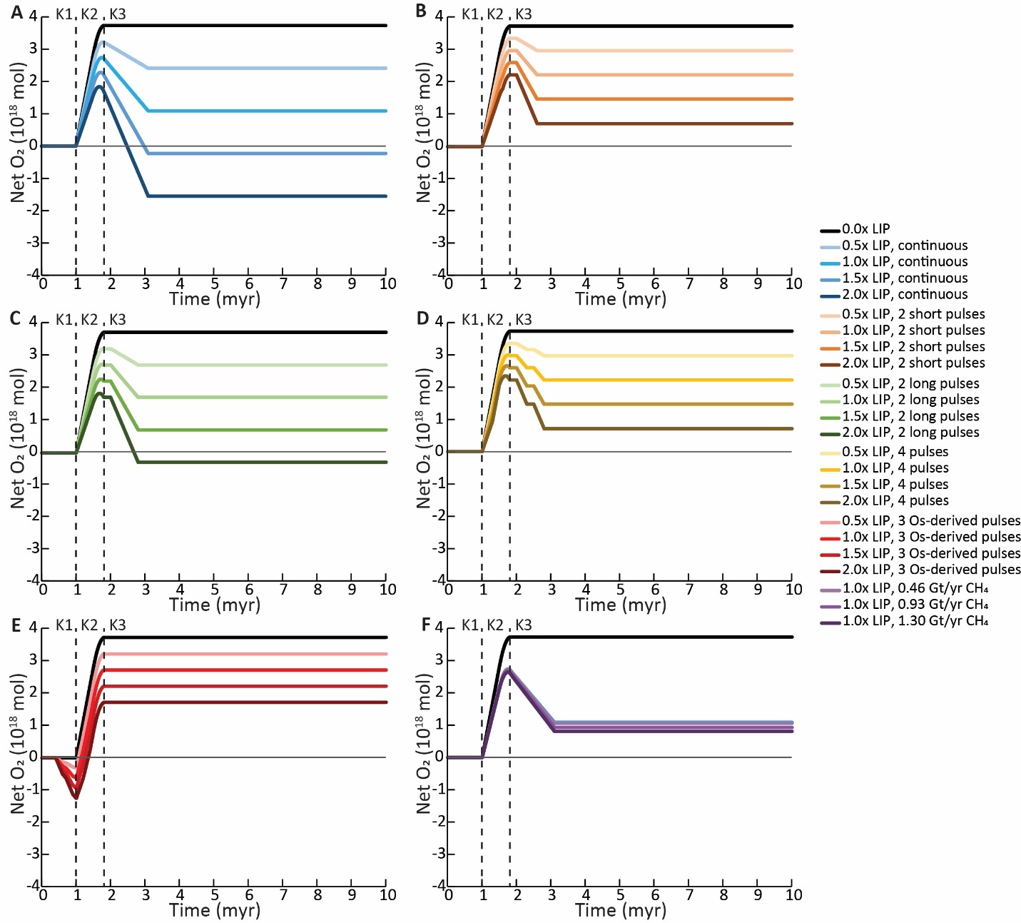
For OAE-2 (supplemental table 4), the total O₂ production from burial of reduced species remained the same across all runs. The net change in O₂ over time was calculated using information derived from the carbon and sulfur isotopic curves for OAE-2 (Owens et al., 2013). This interval is subdivided (fig. 1) into pre-CIE (K1, 1.00 Myr), syn-positive CIE (K2, 0.95 Myr), and post-CIE (K3, 8.05 Myr). There is an increase in excess O₂ produced during K2, releasing 3.73 × 10¹⁸ moles of O₂ across ~0.8 Myr (table 4, figs. 2,3), with similar amounts produced from both reduced carbon (2.04 × 10¹⁸ moles of O₂) and sulfur (1.69 × 10¹⁸ moles of O₂) burial (supplemental table 3).

Various models for the reductant emission loads from HALIP during OAE-2 were analyzed to determine the O₂ production, consumption, and net change (fig. 2, supplemental table 4). These covered a range of sizes, durations, and eruptive styles of the LIP (Kasbohm et al., 2021; Maher, 2001; Sinton & Duncan, 1997). Both continuous and pulsed intervals of volcanic activity were modeled (fig. 2A–D). Alternatively, osmium concentration and isotope indicators of volcanic activity around OAE-2 (Y.-X. Li et al., 2022; Sullivan et al., 2020) may represent pulses of LIP activity and this was also modeled (fig. 2E). A range of reducing material fluxes was considered for the LIP reductants compared to modern mid-oceanic ridge hydrothermal output (supplemental table 1). The abundance of thermogenic CH₄ was also modulated to determine the degree of impact this might have on the O₂ budget (fig. 2F), with minor effect (<0.25 × 10¹⁸ moles of O₂). Overall, the resulting models covered a broad range of net O₂ change across OAE-2, from -1.55 × 10¹⁸ moles of O₂ (net consumption) to 3.22 × 10¹⁸ moles of O₂ produced (table 4, fig. 2, supplemental table 4).

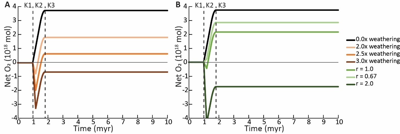
Another set of models was created to determine the effect of oxidative weathering on the O₂ consumption of OAE-2 (fig. 3, supplemental table 4). These primarily cover different rates of weathering, incorporating the silicate weathering rates and intensities of previous studies (Pogge von Strandmann et al., 2013) over 200 kyr (fig. 3A). Another series of sensitivity tests evaluated the effective exponent to describe the relationship between silicate weathering and oxidative weathering, deviating from the value utilized by Berner and Kothavala (2001) in the GEOCARB models from an exponential value of 1.5 (fig. 3B). Overall, the resulting models covered a similar range to the LIP reductants, from -3.47 × 10¹⁸ moles of O₂ (net consumption) to 2.57 × 10¹⁸ moles of O₂ produced (table 4, fig. 3, supplemental table 4).

3.2. T-OAE model results

A carbon model using a recently determined range of organic carbon burial for the T-OAE (Them et al., 2022) was created to determine the degree of O₂ production. The interval surrounding the T-OAE can be subdivided into separate time bins based on the carbon isotope curve, specifically the negative CIE, with labels J1 through J5 (fig. 1) utilized for all other figures and modeling. These bins divide the interval into late Pliensbachian (J1, 1.39 Myr), Toarcian pre-CIE (J2, 1.00 Myr), syn-negative CIE (J3, 0.50 Myr), post-CIE (J4, 2.31 Myr), and return to baseline (J5, 4.80 Myr). Utilizing recently published data of Mo/TOC to recreate organic carbon burial (27.4 × 10¹⁸ to 48.4 × 10¹⁸ moles of carbon buried) over the span of ~1.3 Myr (Them et al., 2022), a positive CIE is modeled with an excursion size of 11.4‰ to 21.8‰, averaging 13.6‰ (fig. 1D). All of these model runs produce a small positive CIE during J2, which increases the isotopic composition by about 0.9‰ to 4.3‰, followed by a major increase to the isotopic maximum during J3, then greatly decreasing to just slightly heavier values (1.7‰ to 2.2‰) than pre-event baseline in J4. At this point, a new positive isotopic plateau is maintained across J4 before returning to the original baseline of 0‰ at J5. Even if isotopically depleted carbon in volcanic CO₂ (~-5‰) from K-F LIP is included in the model (Jones et al., 2016), the effect of this light volcanic carbon is so minute (<0.03‰) that it can only slightly negate the positive CIE produced (supplemental table 5). Thus, the carbon isotopic effect of LIP emissions is ignored for the purposes of these newly derived excursions. An alternative model based on Kemp et al. (2022) was also utilized to estimate total organic carbon burial. These data only focus on the interval of the negative CIE, and therefore all changes were relegated to J3. This calculation provided much smaller estimates for organic carbon burial, which results in a much smaller positive CIE at this time (0.7‰).

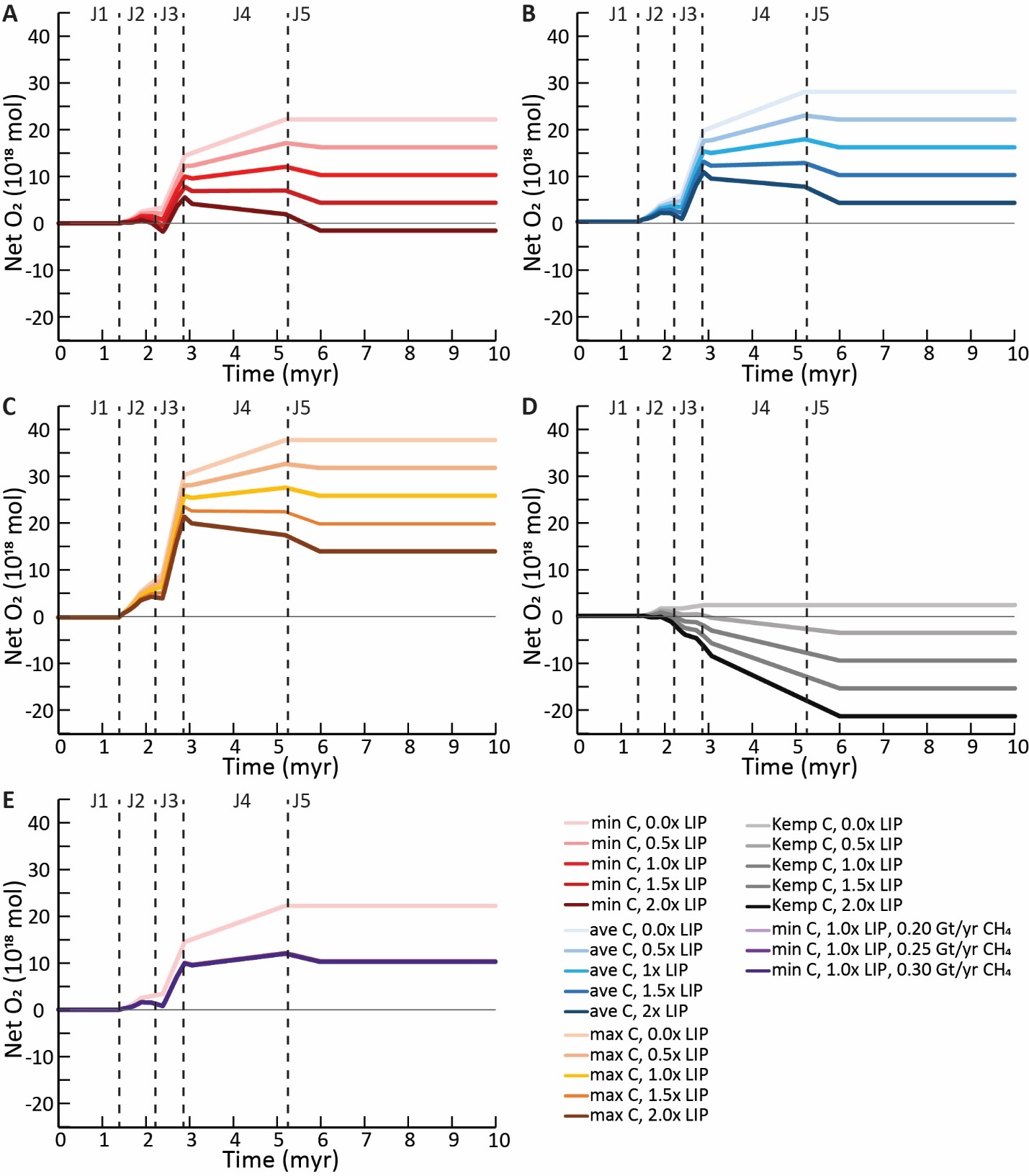
We utilized the methods established for OAE-2 model (described above) with the constraints for the T-OAE (supplemental table 5) to create a model that estimated O₂ change over time using previous models for degree of pyrite sulfur burial for the T-OAE with a conservative, parsimonious estimate of 5 × 10¹⁷ moles (Gill et al., 2011). This resulted in a total of 1.58 × 10¹⁸ moles of O₂ production over 0.5 Myr (supplemental table 3). Conversely, the new T-OAE carbon model based on Them et al. (2022) suggests a very large range of O₂ production due to the wide range of quantities for possible organic carbon burial, with all models indicating a much greater O₂ production via organic carbon burial (20.64 × 10¹⁸ to 36.31 × 10¹⁸ moles O₂ produced) than that determined for pyrite burial (supplemental table 3). Over the course of the increased organic carbon burial interval, lasting ~3.3 Myr, between 22.2 × 10¹⁸ and 37.9 × 10¹⁸ moles of O₂, averaging 27.8 × 10¹⁸ moles of O₂, can be produced from the combined reduced sulfur and carbon burial (fig. 4–6). The model results using Kemp et al. (2022) provide a smaller production of O₂ than even OAE-2, totaling 2.30 × 10¹⁸ moles of O₂ (fig. 4D).

The various model estimates for the T-OAE organic carbon and pyrite sulfur burial were combined with modeled LIP activity based on previously published literature (Burgess et al., 2015; Greber et al., 2020; Kasbohm et al., 2021) to determine O₂ production and consumption and subsequently the overall net change. The LIP activity was varied (supplemental table 5) to account for potential variability in the reductant flux (supplemental table 1). An additional model utilizing the minimum organic carbon burial estimates (Them et al., 2022) was used to modulate the effect of CH₄ inclusion on the oxidative budget of LIPs (fig. 4E), with minor effect (<0.11 × 10¹⁸ moles of O₂). Other tests for CH₄ were employed on the different carbon burial scenarios (supplemental table 5). The resulting models cover a broader range of net O₂ change across the T-OAE as compared to OAE-2, from -21.46 × 10¹⁸ moles of O₂ (net consumption) to 31.95 × 10¹⁸ moles of O₂ produced (table 4).

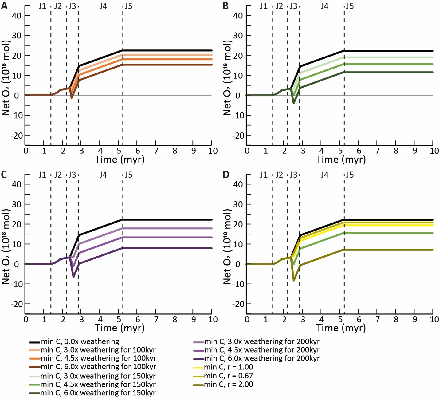
Another set of models were created to determine the effect of oxidative weathering on the O₂ budget of the T-OAE (fig. 5, supplemental table 5). These all use the minimum organic carbon burial flux of Them et al. (2022) as a baseline for comparison. These primarily cover different rates, intensities, and durations of weathering, incorporating the silicate weathering rates of previous studies (Them, Gill, Selby, et al., 2017) to estimate oxidative weathering (fig. 5A–C). Another series of sensitivity tests evaluated the effective exponent to describe the relationship between silicate weathering and oxidative weathering, deviating from the value utilized by Berner and Kothavala (2001) in the GEOCARB models from an exponential value of 1.5 (fig. 5D). Overall, the resulting models covered a smaller range than the LIP reductants, from 3.44 × 10¹⁸ to 19.35 × 10¹⁸ moles of net O₂ produced (table 4, fig. 5, supplemental table 5), partially due to limiting the modeling to a singular carbon burial scenario.

3.3. Combined Results

A final model set was employed for both OAEs combining the LIP reductant and oxidative weathering to determine the total degree of O₂ consumption that might be estimated from these processes. For OAE-2 various tests were employed to estimate the different LIP activity styles but utilized the average of oxidative weathering scenarios (supplemental table 4). This results in a complete utilization of O₂ across all scenarios, with net O₂ between -1.38 and -3.12 × 10¹⁸ moles of O₂ (table 4, fig. 6A, supplemental table 4).

For the T-OAE, various sensitivity tests were employed to examine the average LIP activity and oxidative weathering rate over different organic carbon burial regimes (supplemental table 5). This results in heavy, though not always complete, utilization of O₂ across all scenarios, with a net O₂ consumption and production between -18.46 and 17.12 × 10¹⁸ moles of O₂ (table 4, fig. 6B, supplemental table 5).

4. Discussion

4.1. Assumptions for model creation

These models provide quantitative results, albeit with uncertainties due to ambiguity concerning the model inputs, that can be used as a guide for future investigations related to the fundamental operation of OAEs. However, several of these uncertainties in the presented work should be discussed further, including quantifying the role of the reductant fluxes from LIPs and the estimation of oxidative weathering rates. The production of O₂ due to reduced carbon and sulfur burial requires a simple stoichiometric calculation, but the exact amount of organic carbon and/or pyrite sulfur buried requires mass balance modeling, which is under-constrained for some of the parameters, resulting in multiple solutions. Several methods have been employed to determine the range of potential burial fluxes of reduced species utilizing inorganic carbon isotopes, organic carbon isotopes, global mapping of organic-rich sediments and their geochemical compositions, and other lithologic constraints (Erbacher et al., 2005; Gill et al., 2011; Kemp et al., 2022; Owens et al., 2013, 2018; Raven et al., 2019; Ruebsam et al., 2022; Them et al., 2022). The model presented here primarily incorporates isotopes from inorganic carbon and carbonate-associated sulfate sulfur isotope studies as they more quantifiably represent the burial of their respective reduced compounds at a global scale (Gill et al., 2011; Owens et al., 2013). However, for the flux of organic carbon burial during the T-OAE being more complicated we have utilized a study that incorporates Mo/TOC values because of the inherent limitations when working only with the carbon-isotope record – i.e., sources of light carbon inducing a negative CIE (Ruebsam & Schwark, 2024; Them et al., 2022). Previously determined estimates for reduced species burial used to recreate the respective isotope excursions (Gill et al., 2011; Owens et al., 2013) were used as a starting point for the models presented here (fig. 1), with the focus of this work being on the negative feedbacks that consume O₂. Organic sulfur could also represent a portion of the reduced sulfur burial during these OAEs that would change the absolute degree of O₂ production. However, organic sulfur burial is a poorly constrained during most Phanerozoic OAE intervals, and even those that recognize the potential importance organic sulfur have not quantified its global burial flux (Raven et al., 2019). Therefore, to simplify the models, all reduced sulfur is assumed to be pyrite as it is likely the dominant species, though additional sensitivity tests reveal limited effect from the replacement of pyrite with organic sulfur as a major sulfur species, at greatest ~25% less O₂ produced if all sulfur was buried as organic sulfur instead of pyrite (supplemental fig. 1).

To remedy the issue of a negative CIE during the T-OAE masking the carbon isotopic signal of increases in organic carbon burial, a novel calculation of organic carbon burial inferred from molybdenum geochemistry in organic-rich sediments was utilized (Them et al., 2022). Previous studies on this ratio were used to interpret global marine molybdenum concentration from better established organic carbon burial of OAE-2 (Owens et al., 2016), so the reverse was done for the T-OAE (Them et al., 2022). This provided several potential O₂ production scenarios from carbon burial for the T-OAE (fig. 2A) and the range of tests was done to account for the uncertainty in calculations using this methodology (Berner, 2006; Berner & Canfield, 1989; Owens et al., 2013, 2018). In addition, the estimated positive CIE that this organic carbon burial would have created (excluding input of ¹³C-depleted carbon; fig. 1D) would be greater than any previously documented for the Phanerozoic (Bond & Grasby, 2017; Cramer & Jarvis, 2020). It is possible that the magnitude of the carbon isotope excursion could be modulated by changing the isotopic fractionation of organic matter burial from seawater (Cui et al., 2021). However, a constant typical value of -25‰ was employed in the model for simplicity given the range of uncertainty (Owens et al., 2013). Since the exploration of the size of the positive CIE is not a primary focus of this study, this was not considered further. Nevertheless, emphasis should be put on the minimum organic carbon burial scenarios due to the uncertainty of these estimates.

The minimum organic carbon burial rate creates a large CIE (11.4‰) that places it a slightly larger than the largest Phanerozoic CIEs (< ~10‰) (Cramer & Jarvis, 2020). However, even this consideration means that the negative CIE that is recorded in the geologic record represents far greater input of isotopically light carbon than previous studies have suggested to compensate for the positive CIE that is produced by this buried organic carbon, as suggested by Them et al. (2022). If this Mo/TOC derived estimate for organic carbon burial is utilized there should be a degree of caution since these large CIEs are greater than other known positive carbon excursion of the Phanerozoic (Cramer & Jarvis, 2020). However, this still serves as starting point to compare with later O₂ consumption scenarios to evaluate the effect of the O₂ consumption mechanisms in our models. Therefore, while caution should be applied to this method for calculating global organic carbon burial, the broad trends in modeled T-OAE O₂ budgets are still likely representative but potentially at a higher absolute O₂ levels.

Conversely, an alternative concept for estimating organic carbon burial during the T-OAE utilized a global mapping technique of organic carbon mass accumulation rate of various sediments, primarily from European basins, and comparing that to excess methane carbon input that created the negative CIE fully converting to organic carbon buried (Kemp et al., 2022). The modeled carbon isotope excursion from this burial estimate created an ~0.7‰ positive CIE (supplemental table 5). However, it seems that these values significantly underestimate the total organic carbon burial during the T-OAE (Cohen et al., 2004; Jenkyns, 1988; Kemp et al., 2022; Ruebsam et al., 2022; Ruebsam & Schwark, 2024; Them, Gill, Caruthers, et al., 2017) and, therefore, are less likely to represent the amount of total O₂ production (supplemental discussion). Thus, the minimum carbon burial rate of Them et al. (2022) was the primary estimate used in this study while utilizing various other values in sensitivity tests (fig. 4B; supplemental table 5), especially those not involving LIP activity (fig. 5).

As mentioned above, there are a few uncertainties associated with the flux of materials from LIPs since there is no modern analog for these styles of eruptive events, even when not considering the volatiles released from the intruded country rock. Hotspot volcanism derived from mantle plumes may be most comparable due to having a similar source (Edmonds et al., 2022; Jones et al., 2016; Mason et al., 2021; Self et al., 2008). There are means to approximate the reducing volatile emission rate of hotspot magmatism by comparing the ratios of chemical species in modern emissions and using the better constrained portion of the ratios, such as Cl or SO₂, to determine the unknown half of the ratio, representing emitted compounds, and upscaling for LIP activity (Mason et al., 2021; Self et al., 2008). However, this method has uncertainties due to comparing volatiles to other volatiles, which may not be preserved in the geologic record. Nevertheless, estimates based on these were quantified (supplemental discussion, supplemental table 2) and found to be several orders of magnitude less than that from hydrothermal activity. Therefore, mid-ocean ridge hydrothermal activity has been used as a preferred semi-analogous, first-order estimate for LIP reductants due to being a similarly mantle-derived source of material (Holland, 2002) while also having comparable magnitudes of spatial extent to OAE-like LIPs (supplemental table 1) with broad sensitivity tests on the direct relation to cover various possibilities (fig. 2). Thermogenic release of host rock volatiles from magmatic infiltration has been suggested to have contributed to biogeochemical changes across several recognized intervals and may have contributed to the reductant release of LIPs (Beerling & Brentnall, 2007; Burgess et al., 2017; Green et al., 2022; Jiang et al., 2023). Nevertheless, previous work has not quantified these volatiles for LIPs beyond potential methane (Beerling & Brentnall, 2007), thus the simplified mid-ocean ridge hydrothermal compositions are utilized here, but thermogenic volatiles should be considered in future work.

Another important mechanism for consumption of O₂ is oxidative weathering; however, there are many assumptions that must be made to approximate the effect when there is no current proxy available to accurately quantify global oxidative weathering rates under an oxygen-rich atmosphere. There are several studies that point to a relationship between physical erosion intensity and oxidative weathering intensity (Berner & Kothavala, 2001; Daines et al., 2017; Gabet & Mudd, 2009; Riebe et al., 2003). These are mechanistically linked through the exposure of reduced species to oxidization by the atmosphere. However, the oxidation rate of different species, their age, as well as the degree of exposure necessary to induce oxidative weathering adds complexity this relationship. Additionally, there are no global scale proxies for physical erosion rates in deep-time to the quantifiable degrees needed for modeling exercises presented here (Berner & Kothavala, 2001; Pogge von Strandmann et al., 2023). Changes in other proxies, such as temperature, may provide sufficient means to estimate changes in weathering, though these are unlikely to be directly related to the oxidative weathering changes due to their indirect relationships to the exposure of fresh rock material (Gernon et al., 2024). These also remain several steps removed from providing quantitative estimates of oxidative weathering rates.

Attempts to estimate ancient oxidative weathering for this study rely on the various proxies for silicate weathering (Misra & Froelich, 2012; Pogge von Strandmann et al., 2023) and signals from these proxies may not follow oxidative weathering processes (Kalderon-Asael et al., 2021; Lyons et al., 2014; Misra & Froelich, 2012; Reinhard et al., 2013). Specifically, this correlation is tenuous as there are various inconsistencies between silicate weathering and physical erosion (Daines et al., 2017; Gabet & Mudd, 2009; Pogge von Strandmann et al., 2023; Riebe et al., 2004) that would indicate changes in one may be incongruous with the other. However, many of the studies that have investigated these links focus on local weathering over shorter timespans (< 100 yrs) rather than geologic timescale variability.

When considering oxidative weathering on a global scale and over the long timescales, the GEOCARB model utilizes a simplification of the relationship between silicate weathering and physical erosion (Berner & Kothavala, 2001) that may provide a sufficient approximation. Nevertheless, the uncertain relationship between silicate and oxidative weathering leaves open uncertainties in how they can be related in terms of magnitude as well as their respective response time to other factors (physical erosion, climate, etc.). This includes lag in response time between rock exposure through erosion and subsequent chemical alteration by silicate weathering. The rate of the former is more pertinent to oxidative weathering though not a direct correlative while the latter is what can be approximated through proxy measurements. It is possible that the temperature increase that leads to enhanced silicate weathering can also induce hydrologic changes – e.g., enhanced rainfall and riverine flow – that can then induce increased exposure necessary for oxidative weathering, that is suggested to have occurred during the T-OAE (Them, Gill, Selby, et al., 2017). Additionally, there may be some difference in the response time between silicate and oxidative weathering due to differences in the oxidation rates of organic carbon and pyrite sulfur. While generally these rates are comparable on geologic time scales, processes during lithification can potentially change oxidation rate of rocks of different ages. Thus, in the presented modeling exercises various sensitivity tests were performed to provide a broad range of options for the effect of oxidative weathering, with silicate weathering proxies providing the best feasible quantitative estimates as a baseline for oxidative weathering rates.

4.2. Oxygen production across OAEs

The various assumptions and uncertainties used to create these models do not diminish the first-order implications of both the excess O₂ produced due to organic carbon and pyrite sulfur burial and/or the effect of various reducing mechanisms to consume excess O₂. For OAE-2, we estimate that the total O₂ produced during the entire event through the burial of organic carbon and pyrite is 3.73 × 10¹⁸ moles (figs. 2,3,6), which is ~10% of modern atmospheric O₂ concentrations (36.4 × 10¹⁸ moles). This is a singular value for the produced O₂ across all OAE-2 models with the consumption of O₂ providing the control on the net O₂ due to only one set of organic carbon and pyrite sulfur burial rates being employed. The total O₂ produced by the T-OAE models is between 2.30 × 10¹⁸ and 37.89 × 10¹⁸ moles (figs. 4–6), with the most likely scenarios following the minimum carbon burial option of Them et al. (2022) that produced 22.22 × 10¹⁸ moles O₂ (fig. 4B). These values produce enough O₂ to be on the same size as modern atmospheric content (~60% to 100%). The production of O₂ during the T-OAE and even OAE-2 represent major imbalances in the ocean-atmosphere O₂ budget that must therefore be accounted for. Thus, some mechanism or mechanisms are necessary to limit the excesses accumulation of O₂ in order to maintain an OAE over their known million-year durations (Bond & Grasby, 2017; Jenkyns, 2010).

4.3. LIP impact on oxygen

We considered multiple scenarios of LIP eruptive styles for OAE-2 (Y.-X. Li et al., 2022; Sullivan et al., 2020), and these results are shown in figure 2. The initial set (fig. 2A) includes continuous eruption for the approximate duration of HALIP, which generally induces the largest reductant-driven consumption of O₂ across the OAE-2 LIP reductant scenarios. There are also scenario sets for 2 eruptive pulses, for various durations, and 4 eruptive pulses to account for the uncertainty in the history of HALIP activity (fig. 2B–D). All of these scenarios induce less O₂ consumption compared to continuous eruption scenario. The models based on the osmium isotope record (Y.-X. Li et al., 2022; Sullivan et al., 2020) feature the lowest amount of O₂ removal from LIP reductants (fig. 2E) due to reduced inferred volcanic activity compared to the other scenarios, and these are likely conservative based on the uncertainties assigning specific pulses of volcanism to solely what the osmium isotope proxy records indicate. There are a few scenarios modeled that consume all the produced O₂. This indicates that it is possible to completely remove all O₂ produced from the burial of reduced species simply through LIP activity, though this is unlikely as these are the end-members scenarios with the highest consumption fluxes. All other model runs show a major increase in the amount of O₂ consumed compared to not including LIP activity in the model. There is a consumption of between 0.51 and 5.28 × 10¹⁸ moles of O₂, or 14% to 142% of the produced O₂, through the oxidation of LIP reductants across the modeled scenarios (fig. 2, supplemental fig. 2). Since these modeled sensitivity tests were not randomly selected, a true average is not possible to ascertain, but a median of the different sensitivity tests was determined to provide an approximation of average model output of 1.50 × 10¹⁸ moles, or 54%, of O₂ consumption (table 4). Overall, this reveals there was likely overall increase in net O₂ rather than a balance or loss across the event and therefore that there were likely additional processes beyond LIP activity that consumed O₂.

A smaller set of eruptive scenarios was considered for the T-OAE due to the relatively well-constrained history of volcanism (Burgess et al., 2015; Greber et al., 2020; Kasbohm et al., 2021), only modulating the uncertainty in the amount of reductants released. Additional scenarios were also employed to account for the less-constrained range of carbon burial (supplemental table 5). Similar to OAE-2, all model runs for the T-OAE show significant O₂ consumption by LIP-derived reductants of the O₂ produced from the burial of reduced species. Across the model runs, between 5.94 and 23.76 × 10¹⁸ moles of O₂ were consumed, or 16% to 107% – up to 1033% for some of the models that utilize Kemp et al. (2022)’s lower estimates for carbon burial – of the produced O₂ (fig. 4, supplemental fig. 4). Like OAE-2 model results, an average cannot be completely determined, but the median of these runs was 50% consumption across all the different burial scenarios (table 4). Similar to OAE-2, most of these model runs produced excess O₂ accumulation, but also a significant consumption of O₂ did occur. Therefore, also like the OAE-2 models, additional mechanisms are required to remove the excess O₂ from the ocean-atmosphere system in order to maintain the observed duration of the OAE.

Across the model of both the T-OAE and OAE-2, the effect of CH₄ modulation was small. This species is often invoked as an important driver of climatic change from LIP activity, either as direct volcanic emission or released thermogenically during contact metamorphism of sedimentary rocks (S. J. Baker et al., 2017; Chang et al., 2022; Fendley et al., 2024; Heimdal et al., 2021). This is also one of the several reduced compounds utilized in the calculations (table 1), but CH₄’s importance to global environment change means that there are other constraints on it that could be incorporated. However, even with this importance, when greater proportions of CH₄ were incorporated into the model, only an additional 0.28 × 10¹⁸ moles of O₂ (7%) were consumed for OAE-2 in the highest flux scenario (fig. 2F). For the T-OAE, only 0.11 × 10¹⁸ moles of O₂ (1%) extra were consumed with the greatest flux of CH₄ (fig. 4E). Far greater quantities of CH₄ would need to be introduced to the ocean-atmosphere system to have a more quantitively important impact on the O₂ budget than current estimates for CH₄ released during these events (S. J. Baker et al., 2017; Chang et al., 2022; Fendley et al., 2024; Heimdal et al., 2021).

4.4. Oxidative weathering impact on oxygen

A variety of scenarios were employed for both OAEs to determine the effect of oxidative weathering on the O₂ budget. For OAE-2, the intensity of weathering was modulated across 200 kyr at 2 to 3 times the modern intensity to match the intensity and duration of weathering across this interval as suggested by proxy records (Pogge von Strandmann et al., 2013). This assumes that the exponential relation between silicate and oxidative weathering is 1.5 (Berner & Kothavala, 2001). This results in between 2.52 and 5.77 × 10¹⁸ moles, or 68% to 155%, of O₂ consumption (fig. 3A, supplemental fig. 3A), which is a similar to, though slightly higher than, the range from the LIP activity (median 4.06 × 10¹⁸ moles of O₂, or 106%). The range and median indicate that the expected oxidative weathering on its own could potentially provide the full consumption of excess O₂ during OAE-2. This can be further tested by changing the relation between silicate and oxidative weathering from that used for the GEOCARBSULF models. In this regard, the exponential value of r (eqs 6–7) is modulated between 0.67 and 2 and was modeled with the average weathering intensity of 2.5 times modern intensity (Pogge von Strandmann et al., 2013). This causes a much larger range of effects, between 1.16 and 7.20 × 10¹⁸ moles of O₂, equivalent to 31% to 193%, consumption (fig. 3B, supplemental fig. 3B). Therefore, this relationship can have a greater effect on the O₂ budget, but the potential range from the weathering effect is large due to the uncertainties with implementing this parameter as noted above. Unlike the LIP activity, the majority of scenarios for oxidative weathering during OAE-2 can consume much of the produced excess O₂ (assuming an r value of at least 1.5 is reasonable).

The results for the T-OAE are relatively similar to those from the OAE-2 models. However, they cover a slightly wider range of O₂ consumption scenarios due to longer durations and increases in weathering intensity: between 100 and 200 kyr with 3 to 6 times increased weathering intensities compared to modern weathering (Them, Gill, Selby, et al., 2017). This leaves a larger set of O₂ consumption solutions, between 2.87 and 18.78 × 10¹⁸ moles of O₂, or 13% to 85% consumption (fig. 5A–C, supplemental fig. 5A–C), with a median of 13.44 × 10¹⁸ moles of O₂ consumed, or 40% consumption. Interestingly, unlike the OAE-2 models, the highest-end consumption still does not completely consume the O₂ produced likely due to the higher O₂ produced from organic carbon burial. Compared to the T-OAE results for LIP activity, the O₂ consumed from oxidative weathering generally falls into a similar range. Again, the exponential value (r in eqs 6–7) was modulated using the average scenario of 150 kyr at 4.5 times modern weathering intensity (Them, Gill, Selby, et al., 2017). This ended up ranging between 2.49 and 20.44 × 10¹⁸ moles of O₂, 8% to 89%, consumption (fig. 5D, supplemental fig. 5D), once more indicating that the value for this factor can cause a greater impact than just changes in weathering rate. Furthermore, this mechanism has the potential to consume a large proportion of the excess O₂ produced by the event, but uncertainty in its parameterization point to the need for additional constraints to assess its role in the O₂ budget.

4.5. Comparing and Contrasting OAEs

There are several ways in which the models for these two events differ. The greatest distinction is the amount of O₂ produced and consumed during each event. Production and consumption of O₂ during OAE-2 is approximately an order of magnitude smaller than the T-OAE across nearly all model runs. The difference in production of O₂ can be directly attributed to the larger amount of organic carbon burial predicted for the T-OAE (Them et al., 2022). Smaller quantitative estimates have been suggested (Kemp et al., 2022) and were modeled (fig. 4A) but are likely to be underestimating the total carbon burial (see supplemental discussion). The disparity in carbon burial between the two events is to be expected as the estimated organic carbon to pyrite sulfur burial for the two events are significantly different, with OAE-2 having a C/S (carbon to sulfur ratio) value ranging between 2 and 12 (Hetzel et al., 2009), averaging 5.7 (Owens et al., 2013), while the T-OAE has a range of C/S value from 32 to 62 based on this study (supplemental discussion). This could indicate that there was also a difference in the degree of deoxygenation, with OAE-2’s lower carbon to sulfur burial ratio indicating widespread euxinic (anoxic with water column sulfide) conditions, while the T-OAE’s massive disparity in carbon to sulfur burial potentially indicating more widespread anoxia, but less extensive euxinia, or potentially increased anoxia and carbon burial in non-marine environments (Xu et al., 2017).

Additionally, the greater degree of O₂ production for the T-OAE would require a large removal of O₂ to counterbalance the redox budget and maintain widespread reducing marine conditions (Them et al., 2018, 2022). The larger K-F LIP (Burgess et al., 2015; Greber et al., 2020; Kasbohm et al., 2021) could provide such a supply of greater reducing compounds to the atmosphere and ocean (Kasbohm et al., 2021; Maher, 2001). The difference of magnitude in spatial extent between the smaller HALIP (~200,000 km²) of the Cretaceous (Kasbohm et al., 2021; Maher, 2001) and the larger K-F LIP (~2,000,000 km²) of the Jurassic (Burgess et al., 2015; Greber et al., 2020; Jiang et al., 2023; Kasbohm et al., 2021) is of approximately the same difference as the O₂ produced for each event, assuming similar durations of these LIPs based on the limited and less certain age constraints (Jiang et al., 2023; Kasbohm et al., 2021). This may imply a relationship between the size of the LIP, the LIP-induced climate perturbation, organic carbon and pyrite sulfur burial, the amount of O₂ produced, and the amount of O₂ consumed via reductant load through volcanic activity, as the difference in magnitude of all of these parameters had nearly equal impact for OAE-2 and T-OAE (Bond & Grasby, 2017; Gill et al., 2011; Jiang et al., 2023; Kasbohm et al., 2021; Owens et al., 2013; Pogge von Strandmann et al., 2013; Them, Gill, Selby, et al., 2017; Them et al., 2022). On the other hand, weathering intensities during the T-OAE are estimated to be significantly greater than those prescribed for OAE-2 (Pogge von Strandmann et al., 2013; Them, Gill, Selby, et al., 2017). This difference is not a full order of magnitude and is why the influence of oxidative weathering during the T-OAE is not as impactful (~42% O₂ consumption) when compared to OAE-2 (~88% O₂ consumption). This points to a potentially greater significance of the LIP reductants in the O₂ budget, at least for these two OAEs, though oxidative weathering and other processes should not be discounted.

It should also be noted that there is an order-of-magnitude difference in biological extinction/turnover that occurred during OAE-2 and the T-OAE. OAE-2 is associated with several minor extinctions, coined as turnover events by some, that were localized and affected specific, limited groups of organisms (Coccioni & Galeotti, 2003; Elder, 1989). Meanwhile, the T-OAE is associated with a major extinction event that affected various faunal groups globally (Bond & Grasby, 2017; Caruthers et al., 2013; Morten & Twitchett, 2009; Wignall et al., 2006, 2010). This difference in extinction rate between the two events would match closely to the scalar relationship between LIP size and changes in net O₂. Therefore, these shifts in O₂ budget could be correlative to the size of extinction and such factors should also be considered when looking at other extinction events.

4.6. An additional parameter – Phosphorous cycling

Overall, these sensitivity tests suggest OAEs are prone to producing large quantities of O₂ through the burial of reduced compounds that are likely counterbalanced by LIP activity and oxidative weathering. Both processes under most scenarios consume enough O₂ to maintain deoxygenation (fig. 6). However, additional processes may also bear on the O₂ budgets of these events (supplemental discussion).

One notable factor to consider is changes in the cycling of phosphorus during OAEs which may also be able to extend the duration of deoxygenation and further decrease the excess net O₂. Specifically, phosphorous absorbed onto the surfaces of Fe-oxide minerals is released into seawater when these oxides are dissolved as anoxic conditions become prevalent. This provides an important flux of this biolimiting nutrient to the water column that can stimulate primary productivity, which in turn may induce more O₂ production in the shorter term but lead to greater deoxygenation and additional Fe-oxide dissolution in the longer term (Gernon et al., 2024; Reershemius & Planavsky, 2021; Van Cappellen & Ingall, 1994). This positive feedback loop will then follow until there are insufficient Fe-oxides to dissolve or the extent of anoxia on the ocean floor reaches some maximum dictated by other processes. This feedback loop would work with the mechanisms proposed in this study to extend the duration of deoxygenation, especially if LIPs and/or weathering also provide additional sources of phosphorus. This phosphorous feedback requires large amounts of Fe-oxides initially present for the feedback cycles to persist for several hundred thousand years and tracking this process in the sedimentary record is difficult due to a lack of appropriate proxies. One source of physical evidence is the eventual accumulation of Mn-rich sediments in the oxic shallow waters near to these anoxic regions, often referred to as “bathtub rings” like found in the Black Sea (Force & Cannon, 1988). These Mn-rich sediments are likely the product of Fe-Mn-oxide dissolution under anoxic conditions, though their accumulation and preservation is discontinuous and therefore do not provide a quantitative estimate for Fe-oxide dissolution during OAEs (Gambacorta et al., 2024).

Chemical weathering may also enhance phosphorous delivery via the weathering of basaltic rocks (Gernon et al., 2024) linking LIP activity and oxidative weathering as a potential nutrient source in additional to their role as O₂ sink. Constraining and quantifying changes to these processes in the geologic past beyond modeling due to the limited proxies for phosphorous cycling (Gernon et al., 2024). Regardless, this work and previous studies show that the LIP-reductant load (Sinton & Duncan, 1997), enhanced oxidative weathering (Berner, 2006; Berner & Canfield, 1989; Berner & Kothavala, 2001), and/or phosphorous cycling (Gernon et al., 2024; Reershemius & Planavsky, 2021) certainly played a role in the O₂ budgets of these events.

5. Conclusions

We provide a novel modeling study of the production and consumption of O₂ across two Mesozoic oceanic anoxic events. The burial of organic carbon and pyrite sulfur across OAE-2 and the T-OAE could have produced large amounts O₂ that approached the modern content of the atmosphere. For both events, input of reduced chemical species from LIPs could provide enough reductive flux to consume much of the excess produced O₂. Similarly, oxidative weathering can also consume a major portion of the produced O₂. There is variability across all the modeled scenarios in how much O₂ could be consumed, with the two mechanisms combined typically consuming the majority of excess O₂. This consumption of O₂ can provide a mechanism to help explain the protracted duration of OAEs. It is possible, based on some of the scenarios, that these processes conspire to result in net loss of O₂ from the ocean atmosphere system. In that case, additional processes provide an important underlying mechanism for an OAE. However, more accurate quantification, timing and duration is required to better constrain this relationship.

The order-of-magnitude difference in O₂ production and consumption between OAE-2 and the T-OAE matches the magnitude difference between the size of their respective LIP and the extinction rates observed with these two events. There are many other factors and processes, such as climate and marine productivity, as well as other elemental cycles, that were likely affected by the O₂ budget of OAEs and exploring these are avenues of future study.

There are other Phanerozoic C and S cycle perturbations based on large isotopic excursions that are not known to be tied to LIP emplacement (Bond & Grasby, 2017; Cramer & Jarvis, 2020; Jenkyns, 2010), and thus, understanding the O₂ budgets of these events likely require invoking additional mechanisms to produce and limit O₂. Further, there are intervals of LIP activity that have no significant oceanic anoxia associated with them (Jiang et al., 2023; Kasbohm et al., 2021). This dichotomy emphasizes oxidative weathering and/or other processes on the global O₂ budget are factors that need to be considered for these events and the effect of LIP source reductants should also not be overlooked. Sources of variability in the response of the ocean and atmosphere during these events are likely the result of the particular starting state of the ocean atmospheric system: the spatial or temporal variability of physical processes in the oceans, the climate, other biogeochemical mechanisms, etc. (Berner & Kothavala, 2001; Gernon et al., 2024; Reershemius & Planavsky, 2021). However, the reductants introduced by LIPs and effects of oxidative weathering should be considered when studying these events.

The models presented here provide a framework for understanding of the processes that should be involved, but this work highlights where more constraint is needed to improve our understanding these events. Better estimates of LIP reductant loads, through better estimates of the elemental budgets of LIPs or better analogs for the release of material across the spatial extents of igneous provinces, would aid in constraining their impacts on O₂ budgets. Identification of the LIP(s) responsible for OAE-2 and timelines for their eruptive activity would sharpen our estimates for O₂ consumption from igneous-source reductants. Conversely, our understanding of the O₂ budget of the T-OAE would benefit from an improved approximation of the event-driven organic carbon burial. Additionally, the quantification of oxidative weathering needs better overall constraints especially given our best weathering proxies relate to silicate weathering, which is likely not directly comparable. Lastly, the impact of the phosphorous and iron cycles and their feedbacks across OAEs need to be better tracked to determine their role in the O₂ budget. All this future work would not only improve the models needed to determine the redox budgets across these anoxic events, but also constrain the mechanisms involved in the development and termination of OAEs more generally.

Acknowledgments

This work was funded by grants from the National Science Foundation (EAR-2026926) to JDO and BCG, Alfred P. Sloan Foundation FG-2020-13552 (JDO), and the FSU EOAS Winchester Fund for graduate student support (SMN). We greatly appreciate the contributions and suggestions from our two reviewers and the associate editor.

Author Contributions

SMN was the primary author and created the models utilized in this study. BCG and JDO provided portions of models from previous studies to be utilized. TRT contributed additional data sets to approximate important missing parameters. BCG, JDO, SAY, SMN, and TRT all provided insights and parameterizations for the models and contributed to editing of the text. JDO, BCG, and SMN all contributed some funding for the project.

Conflicts of Interest

The authors declare no conflict of interest.

Supplementary Data

https://doi.org/10.17632/vgt7hjmnrs.1

Editor: C. Page Chamberlain, Associate Editor: Jonathan L. Payne