A Micromechanical Model for Mineral Replacement Reactions and Associated Deformation: From Pore Clogging to Solid Volume Increase

1. Introduction

Coupled chemical reactions and deformation play a crucial role in understanding the dynamic processes that shape the Earth’s surface and subsurface. In geology, these processes are fundamental for explaining the formation of rocks, minerals, and the overall evolution of our planet. For instance, the process of mountain building, known as orogeny, involves the deformation of rocks due to tectonic forces. During this process, chemical reactions occur within the rocks, leading to their metamorphism or transformation into new minerals (e.g., Schenker et al., 2015). Melt transport and chemical differentiation, essential for oceanic crust formation and intraplate volcanism, are aided by mechanical compaction and decompaction (e.g., Bessat et al., 2022). Deformation at tectonic plate boundaries involves coupling between rock deformation, fluid flow, and metamorphic reactions, where a propagating reaction front causes an effective, reaction-induced weakening of the heterogeneous rock (Schmalholz et al., 2020). Understanding coupled chemical reactions and deformation is crucial for predicting and mitigating geological hazards. Chemical reactions within fault zones can affect the strength and behavior of rocks, influencing their ability to slip or fracture during seismic events (e.g., Rohmer et al., 2016). In civil and petroleum engineering, chemical reactions lead to the degradation of the building materials and cement when in contact with carbon dioxide or strong acids (Fabbri et al., 2009; Lesti et al., 2013; Vrålstad et al., 2019). In environmental engineering, CO₂ storage in mafic and ultramafic rocks has gained attention as a potential solution for mitigating greenhouse gas emissions. These rocks can react with CO₂ through mineral carbonation, which converts CO₂ into solid mineral forms, providing long-term CO₂ storage options. However, a debate surrounds the possibility of achieving a complete reaction within these rocks and the role of fracturing in enhancing this process (Kelemen & Hirth, 2012; Snæbjörnsdóttir et al., 2020; Van Noort et al., 2017; Yarushina & Bercovici, 2013).

The models of coupled processes incorporate equations for fluid flow, chemical transport, and mechanical deformation. These equations are governed by the principles of conservation laws in thermodynamics, ensuring mass, momentum, and energy conservation throughout the system (Malvoisin et al., 2015; Vrijmoed & Podladchikov, 2022; Yarushina & Podladchikov, 2015). However, to fully describe the system’s behavior, a complete set of governing equations is required. This is achieved through the development of closure equations, which establish the necessary additional relationships between key variables, such as stress and strain, porosity and permeability, porosity and reaction, porosity and effective pressure, and reaction rate and temperature. Differences in the formulation of closure equations can lead to significant variations in model predictions (Malvoisin et al., 2021). These closure equations are either obtained by extrapolating the experimental data or derived from micromechanical models, which consider the processes occurring at the scale of individual grains or particles.

Mineral replacement reactions have traditionally been explained by solid-state mechanisms, where one phase transforms into another via volume diffusion through the crystal lattice. However, such processes are typically too slow under geological conditions unless very high temperatures are present, as diffusion rates increase rapidly with temperature. When fluid is involved, mineral replacement is more effectively described by a coupled dissolution and reprecipitation process (A. Putnis, 2009). Two major types of fluid-mediated replacement models have been proposed. The first type, often referred to as interface-coupled dissolution-precipitation, emphasizes chemical control at the reaction front. In this model, the parent mineral dissolves at the interface, creating a localized supersaturation that promotes nucleation and growth of the product phase (Anderson et al., 1998; A. Putnis, 2002, 2009). This mechanism relies on the chemistry of the boundary layer fluid and diffusion across short distances, explaining pseudomorphic textures through close spatial coupling of dissolution and precipitation. The second class of models includes those that incorporate mechanical or stress-driven processes. Some models propose that a growing product phase exerts stress on the adjacent parent mineral, the so-called “force” of crystallization, inducing pressure-driven dissolution (Fletcher & Merino, 2001; Merino & Dewers, 1998; Schmid et al., 2009). These models account for rheological feedback between crystal growth and the mechanical response of a surrounding rock matrix, particularly under confined or non-hydrostatic conditions. In contrast, classic pressure solution models (Rutter, 1976; Weyl, 1959) describe mineral dissolution at stressed grain contacts with subsequent diffusion and reprecipitation at distant, unstressed surfaces. Here, dissolution and precipitation are often spatially and temporally decoupled, and the rate-limiting step is typically solute diffusion through thin fluid films. While interface-coupled models effectively explain the role of fluid composition, supersaturation, and boundary layer transport, they may neglect the mechanical constraints present in confined systems. Pressure solution models predict a very limited extent of reaction due to loss of porosity and reactive surface area (Malvoisin et al., 2017). Yet, field observations report that natural rocks can undergo 100% hydration/carbonation (Kelemen & Matter, 2008). The stress-based models of Fletcher and Merino (2001); Merino and Dewers (1998), and Schmid et al. (2009) consider alterations and deformation due to mineral growth but do not consider their feedback on porosity evolution. Recent experimental and observational studies suggest that mineral replacement is associated with both the change in the solid volume and porosity (Malvoisin et al., 2020; A. Putnis, 2002; C. V. Putnis et al., 2021).

Thus, the plausible solution is to combine both approaches by considering a microscale model where porosity changes and mineral replacement will be combined and driven by changes in the fluid chemistry. Microscale models are often based on simplified analytical solutions obtained for idealized conditions that may not capture the full complexity of real-world situations. For example, it is often assumed that deformations that develop in the rock are small and obey the linear elastic law. At the same time, thermodynamic databases such as that of Holland and Powell (1998) present a nonlinear Murnaghan equation of state (EOS) for the deformation of common minerals. Observations show that reaction-induced volume change can be as large as 30–70% (Lyu et al., 2015; Malvoisin et al., 2020). One way to tackle this discrepancy is to derive nonlinear finite strain analytical solutions. However, it may not always be possible, and the results obtained will be too cumbersome to be practical. Another approach is to keep simplified solutions but compare them with nonlinear finite strain numerical simulations to assess their validity (Moulas et al., 2023). If the analytical solution matches the results of the numerical simulation, it provides confidence in the accuracy of the mathematical model.

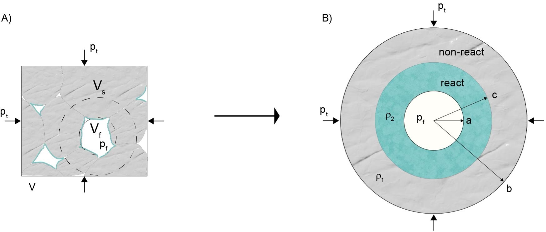
In this work, we present a new analytical model and supporting numerical results that extend the micromechanical approach introduced in Yarushina et al. (2023), with key enhancements. Building on that framework, we derive macroscopic compaction relations for reacting porous materials by accounting for elastic, viscous, and plastic deformation of the solid matrix. Our approach accounts for the influence of chemical reactions on microscale deformation, and crucially, incorporates plastic failure or fracturing ahead of the reaction front. This feature improves fluid access to reactive surfaces and naturally limits unrealistic stress buildup within the evolving microstructure. A central contribution of this study is the development of an effective rheology in which porosity evolves as a function of the relative deformation rates of the solid and pore volumes. This provides a more general and physically grounded framework for exploring the coupled evolution of deformation and reaction in porous media. Our model targets mineral replacement reactions occurring under deforming conditions, as illustrated in figure 1. In this setting, a reactive fluid within the pore space interacts with the solid matrix to form a product phase with different mechanical and transport properties. The analytical formulation is developed within a 2D plane strain approximation, appropriate for systems with cylindrical symmetry, and can be extended to fully 3D cases in an analogous manner. The inclusion of fracturing mechanisms allows the model to realistically capture porosity generation, enhanced transport, and stress relaxation near the reaction front. To complement the analytical model, we present nonlinear finite-strain numerical simulations that validate and extend the analytical results. These numerical investigations are an important addition to the work of Yarushina et al. (2023), broadening the model’s applicability beyond linear regimes. Finally, we formulate a closed, macroscopic system of equations that governs the coupled evolution of fluid flow, reaction, and deformation. This framework is broadly applicable to both natural systems and engineered processes involving reactive porous materials.

2. Effective rheology of reacting porous media

In this section, we follow the micromechanical procedure developed in Yarushina et al. (2023) to define an effective medium representation of a reactive porous material undergoing deformation. Our goal is to derive macroscopic rheological laws that capture the essential coupling between chemical reactions and deformation within a fluid-saturated porous medium. The model is constructed to explore the range of behaviors between two end-member regimes: porosity-preserving and porosity-clogging mineral replacement reactions. Rather than representing discrete modes, these two regimes emerge naturally from the relative rates of deformation and reaction and thus define a continuous spectrum of behaviors.

We consider a representative elementary volume (REV) of a porous matrix, fully saturated with a single, reactive fluid. Chemical alteration is assumed to be driven by a fluid phase that is out of equilibrium with the surrounding solid, initiating a reaction at the fluid-solid interface and progressing into the solid matrix (fig. 1A). The model assumes isothermal conditions and does not account for thermal stress. We acknowledge that the reactive surface area and mineral distribution are critical in natural settings; however, our model simplifies these complexities by assuming a uniform reactive interface. This simplification allows us to focus on the coupled evolution of porosity, reaction, and mechanical deformation, and should be viewed as a first-order approximation of more complex, heterogeneous systems.

We idealize the geometry of the REV as a 2D array of cylindrical pores surrounded by concentric shells of deformable solid (fig. 1B). This 2D formulation serves as a computationally tractable abstraction of the 3D problem. While the dimensionality reduction simplifies mathematics, it implies that the pores behave as infinitely long cylinders in the out-of-plane direction. This assumption limits the model’s ability to capture certain 3D features such as complex non-isotropic stress states or complex pore shapes. Nonetheless, comparisons with experimental data and prior modeling efforts suggest that this cylindrical approximation captures the essential mechanics of porosity evolution and solid deformation (Carroll & Holt, 1972; Yarushina et al., 2020; Zimmerman, 1991). Zimmerman (1991, p. 91) and Mavko et al. (1998, p. 42) suggest that while different pore shapes affect the numerical coefficients, the functional dependence of rock compressibility on stress and porosity remains the same across a wide range of pore geometries. The model allows for fluid mobility across the porous network, assuming interconnected pores that facilitate mass transport between neighboring regions. We do not explicitly model fluid flow but assume that the fluid is always present in the pore space and that reaction rates are not limited by large-scale fluid supply but by local interface kinetics and deformation.

Geomaterials such as basaltic rocks and cementitious materials exhibit both instantaneous elastic deformation and time-dependent viscous creep, as documented in experimental studies (Heap et al., 2011; Nermoen et al., 2015; Neville et al., 1983; Sabitova et al., 2021; Wolterbeek et al., 2016; Yarushina et al., 2021). We incorporate these two deformation mechanisms as limiting cases of the solid matrix response. To define the mechanical loading in the model, we apply boundary conditions at the inner and outer surfaces of the cylindrical volume. In the viscous formulation, the fluid pressure $p_{f}$ is applied at the pore wall, while the total confining pressure $p_{t}$ is applied at the outer boundary (fig. 1B). In the elastic model, the corresponding pressure rates, ${\dot{p}}_{f}$ and ${\dot{p}}_{t}$, are prescribed at the internal and external boundaries, respectively. This difference arises because viscous constitutive relations are formulated in terms of stresses and velocities, so boundary pressures directly influence stress and flow. In contrast, the elastic constitutive equations are rate-based, where velocities are related to stress rates rather than stresses themselves, requiring the specification of pressure rates at the boundaries. These boundary conditions govern the stress evolution within the solid shell and control its mechanical response to ongoing reaction and deformation.

We consider reactions where the mass of immobile species is conserved. For instance, during the hydration of periclase, magnesium and oxygen remain in the solid phase despite compositional changes. Although these elements remain immobile, ensuring their conservation within the solid matrix, the overall mass of the solid increases as water is incorporated to form brucite. Similarly, during the hydration of olivine, silicon, magnesium, and iron remain immobile as they are retained within the newly formed hydrated mineral, serpentine. In the carbonation of portlandite, calcium and oxygen are immobile species, remaining in the solid phase as portlandite transforms into calcite. In addition to these mineral alteration reactions, various other types of reactions also conserve the mass of immobile species, provided they remain in the solid phase without undergoing dissolution or volatilization. Additional examples can be found in Appendix A.

Macroscopic porosity in the model is characterized by the ratio of the fluid volume, V_f, to the total volume, V (see table 1 for the list of notations). For cylindrical pores, it can be defined in terms of the pore radius, a, and the outer radius of a cylindrical shell, b, (fig. 1), so that

$$\varphi = \frac{V_{f}}{V} = \frac{a^{2}}{b^{2}} \tag{1}$$

The macroscopic extent of reaction, ξ(t), can be defined as the volume fraction of the reacted portion of the solid:

$$\xi(t) = \frac{c(t)^{2} - a(t)^{2}}{b(t)^{2} - a(t)^{2}} \tag{2}$$

Changes in ξ(t), and consequently in c(t), are influenced by mass transfer or diffusion in cases where the reaction occurs under thermodynamic equilibrium or is extremely fast. In such cases, ξ(t) should be determined by solving the full set of equations governing mass and momentum balance (see Sections 3 and 4). For reactions governed by chemical kinetics, the time derivative of the extent of reaction corresponds to the reaction rate, which can be expressed using various kinetic laws. The bulk volume strain is a function of changes in pore volume and changes in the volume of the solid matrix. These together lead to changes in the total volume. Thus, only two equations are needed to describe the expansion or compaction of porous materials. For the micromechanical approach, it is convenient to consider changes in porosity and the total volume. It is practical to rewrite the porosity equation in the following differential form used in further derivations:

$$\frac{d\varphi}{dt} = \frac{2\varphi}{a}\frac{da}{dt} - \frac{2\varphi}{b}\frac{db}{dt} = 2\varphi\left( \left. \ \frac{v}{r} \right|_{r = a} - \left. \ \frac{v}{r} \right|_{r = b} \right) \tag{3}$$

where v is the radial velocity of the solid. The applied far-field pressure, pore pressure, and ongoing chemical transformations induce non-uniform deformation on the microscale. Macroscopic, or averaged, volumetric deformation, is determined by changes in the total volume of the Representative Elementary Volume (REV):

$$\frac{d\varepsilon}{dt} = \frac{1}{V}\frac{dV}{dt} = 2\left. \ \frac{v}{r} \right|_{r = b} \tag{4}$$

Figure 1.Schematic model for mineral replacement reaction. (a) The total volume, $V$, consists of solid, $V_s$, and pore fluid, $V_f$. The reaction starts at the fluid-solid contact and progresses into the solid volume (green). The fluid pressure, $p_f$, and the external total pressure, $p_t$, act on the volume in a viscous model. In the elastic model, the rates of fluid pressure, ${\dot{p}}_{f}$, and total pressure, ${\dot{p}}_{t}$, are prescribed at the internal and external boundaries of the volume, respectively. (b) Representative Elementary Volume (REV) for mineral replacement reaction in porous media. The reaction starts around the cylindrical pore and progresses into the initial solid phase. Reacted and non-reacted materials have different densities and mechanical properties. Pore radius, $a$, and radius of REV, $b$, are determined by porosity. A reaction rim of radius $c$ grows into the shell starting from the pore radius, $a$.

2.1. Elastic adjustment of the matrix

The constitutive equations for a linear elastic material relate the shear strain rate to the shear stress and the volumetric strain rate to the mean stress:

$$\frac{\partial v}{\partial r} - \frac{v}{r} = \frac{{\dot{\sigma}}_{r} - {\dot{\sigma}}_{\theta}}{2G}\mspace{6mu} \tag{5}$$

$$\frac{\partial v}{\partial r} + \frac{v}{r} = \frac{{\dot{\sigma}}_{r} + {\dot{\sigma}}_{\theta}}{2K} \tag{6}$$

where G is the elastic shear modulus, K is the elastic bulk modulus, $\sigma_{r}$ and $\sigma_{\theta}$ are the radial and tangential components of the stress tensor at the microscale. The dot represents the Lagrangian time derivative. Both reacted and non-reacted parts of the solid volume must be in mechanical equilibrium and satisfy the force balance equation

$$\frac{\partial\sigma_{r}}{\partial r} + \frac{\sigma_{r} - \sigma_{\theta}}{r} = 0 \tag{7}$$

These equations must be satisfied in the solid’s reacted and nonreacted parts. Conservation of momentum requires normal stress to be continuous at the reaction front. Assuming that the mass of immobile species is conserved at the reaction front, as in hydration or carbonation reactions, the following jump condition must be satisfied:

$$\left. \ \left( \rho_{1}X_{1}v_{1} - \rho_{2}X_{2}v_{2} \right) \right|_{r = c} = \frac{dc}{dt}\left( \rho_{1}X_{1} - \rho_{2}X_{2} \right) \tag{8}$$

where X is the concentration of the immobile component. Index 1 denotes quantities in the non-reacted phase, and index 2 marks the reacted phase. This jump condition is similar to the classical Stefan condition in thermal problems (Mainguy & Coussy, 2000; Rubinshteĭn, 1971), but it arises from mass balance rather than energy balance.

Equations – form a system of three equations with three unknowns: $v$, $\sigma_{r}$, and $\sigma_{\theta}$. We solve these equations separately for the non-reacted and reacted parts of the volume, ensuring that $\sigma_{r}$ is equal to the fluid pressure at the pore boundary and the total pressure at the external boundary, as illustrated in figure 1. The remaining condition at the interface between two regions is provided by the equation . By substituting c(t) with ξ(t) using the equation, we obtain the following velocities:

$$v_{1} = - \frac{1}{2r\widehat{G}}\left( \begin{array}{l} \frac{b^{2}}{b^{2} - a^{2}}A_{11}\frac{dp_{e}}{dt}\\ \quad + A_{12}\frac{dp_{f}}{dt} + A_{13}\frac{d\xi}{dt} \end{array} \right)\tag{9}$$

$$v_{2} = - \frac{1}{2r\widehat{G}}\left( \begin{array}{l} \frac{b^{2}}{b^{2} - a^{2}}A_{21}\frac{dp_{e}}{dt}\\ \quad + A_{22}\frac{dp_{f}}{dt} + A_{23}\frac{d\xi}{dt} \end{array} \right) \tag{10}$$

and stresses around the pore

$${\dot{\sigma}}_{r}^{1} = - \frac{1}{\widehat{G}r^{2}}\left( \begin{array}{l} \frac{b^{2}}{b^{2} - a^{2}}B_{11}\frac{dp_{e}}{dt} + B_{12}\frac{dp_{f}}{dt}\\ \quad + (b^{2} - r^{2})\xi B_{13}\frac{d\xi}{dt} \end{array} \right) \tag{11}$$

$${\dot{\sigma}}_{\theta}^{1} = - \frac{1}{\widehat{G}r^{2}}\left( \begin{array}{l} \frac{b^{2}}{b^{2} - a^{2}}C_{11}\frac{dp_{e}}{dt} + C_{12}\frac{dp_{f}}{dt}\\ \quad - (b^{2} + r^{2})\xi C_{13}\frac{d\xi}{dt} \end{array} \right) \tag{12}$$

$${\dot{\sigma}}_{r}^{2} = - \frac{1}{\widehat{G}r^{2}}\left( \begin{array}{l} \frac{b^{2}}{b^{2} - a^{2}}B_{21}\frac{dp_{e}}{dt} + B_{22}\frac{dp_{f}}{dt}\\ \quad + (r^{2} - a^{2})(1 - \xi)B_{23}\frac{d\xi}{dt} \end{array} \right) \tag{13}$$

$${\dot{\sigma}}_{\theta}^{2} = - \frac{1}{\widehat{G}r^{2}}\left( \begin{array}{l} \frac{b^{2}}{b^{2} - a^{2}}C_{21}\frac{dp_{e}}{dt} + C_{22}\frac{dp_{f}}{dt}\\ \quad + (1 - \xi)(r^{2} + a^{2})C_{23}\frac{d\xi}{dt} \end{array} \right) \tag{14}$$

where $p_{e} = p_{t} - p_{f}$ is the effective pressure. All the coefficients in equations – are dimensional shorthand notations and do not represent meaningful physical quantities. A summary of these coefficients is provided in Appendix B.

2.1.1. Effects of nonlinearity and comparison with the numerical solution

The volumetric behavior of minerals is widely recognized to possess inherent nonlinearity, as acknowledged by Angel et al. (2018) and Moulas et al. (2023). Thermodynamic databases commonly employ nonlinear elastic equations of state (EOS) to describe the behavior of minerals (Holland & Powell, 1998, 2011). The extent of strain depends on the nature and magnitude of the reaction, as well as the mechanical properties of minerals. Various chemical reactions can generate finite strain, including hydration or carbonation reactions, that involve the addition of water or carbon dioxide molecules to compounds, leading to changes in molecular structure and volume. Notably, Malvoisin et al. (2020) observed a volume change of 59% to 74% during the serpentinization of dunite samples collected at depth during the Oman Drilling Project. Similarly, Lyu et al. (2015) reported data on significant shale swelling of up to 30% due to water adsorption.

We use numerical simulations to study the effect of finite strain and material nonlinearity of the minerals on the porosity and volume changes. Our numerical code is based on the Lagrangian hyperelastic formulation of Lurie (1990), Levin et al. (2013), and Levin et al. (2021). Numerical aspects of its implementation are described in Moulas et al. (2023). The nonlinear elastic behavior in our numerical model is described in terms of the strain energy function, W, as follows:

$$\sigma_{j} = \frac{\lambda_{j}}{i_{3}}\frac{\partial W}{\partial\lambda_{j}} \tag{15}$$

$$\begin{aligned} W &= 2G(i_{1} - 3)\\ & \quad + \frac{K_{0}}{K^{\mathstrut'}(K^{\mathstrut'} - 1)}\left\lbrack i_{3}^{1 - K^{\mathstrut'}} + (K^{\mathstrut'} - 1)i_{3} \right\rbrack \end{aligned}\tag{16}$$

Here, $\sigma_{i}$ are the true (Cauchy) stress components, $\lambda_{i}$ are the principal stretches, and $i_{1}$, $i_{3}$are the invariant forms defined as

$$i_{1} = (\lambda_{1} + \lambda_{2} + \lambda_{3}) - 3\sqrt[3]{i_{3}},\quad i_{3} = \lambda_{1}\lambda_{2}\lambda_{3} \tag{17}$$

Equations and reduce to the isothermal Murnaghan EOS for pure-hydrostatic compression. $G$, $K_{0}$ and $K^{\mathstrut'}$ are the nonlinear material parameters. In the linear limit, $K_{0}$, and G reduce to the usual bulk and shear moduli.

In the numerical examples presented below, we set both the total confining pressure $p_{t}$ and fluid pressure $p_{f}$ to zero at the boundaries. This choice ensures that the resulting stresses are driven solely by the extent of the chemical reaction and associated deformation, rather than by externally imposed boundary loads. This approach provides conservative estimates that can be interpreted as perturbations from the geological stresses developed due to natural confinement. It is important to emphasize that the derived analytical solution is general and allows for arbitrary boundary pressures. Figure 2A and 2B illustrate increments of stress and displacements within the REV computed for nonlinear hyperplastic materials under traction-free boundary conditions when $p_{f} = p_{t} = 0$ corresponding to a small increase in reaction progress from $\xi = 0.4$ by the amount given by $d\xi$. The incremental linear elastic analytical solution is also shown for comparison. The incremental nature of the analytical solution implies that the final values of the external loads and reaction progress are reached in several steps by applying small incremental changes to the external parameters and evaluating how the internal parameters, i.e., stress and displacement change in response to the small loads. This approach gives an improved estimate in case of large strains in comparison with small-strain elastic solutions. Figure 2A and 2B show a comparison of the numerical and analytical solutions for two different values of incremental steps in solution, given as increments in the reaction progress $d\xi$ at zero fluid and total pressures. They show that the analytical solution obtained with small incremental steps $d\xi = 0.01$ is indistinguishable from a fully nonlinear large-strain numerical solution. Larger increments in the analytical solution $d\xi = 0.1$ lead to minor deviations from the nonlinear numerical solution. Moreover, comparison of numerical solutions obtained for two different values of the nonlinear parameter $K^{\mathstrut'}$, show that nonlinearity has an insignificant influence on the solution. The material’s response to the applied load and reaction progress are mainly controlled by the linear elastic bulk and shear moduli.

Figure 2.Comparison of elastic stress and displacement increments within REV: incremental analytical vs. fully nonlinear numerical solutions corresponding to a small increase in reaction progress from $ξ=0.4$ by the amount of $dξ$ as indicated on the figures. All simulations were performed at $\varphi = 0.15$, $\frac{\rho_{2}}{\rho_{1}} = 0.8$,$\frac{G_{2}}{G_{1}} = 0.7$, $\frac{K_{1}}{G_{1}} = 3.3$.

2.2. Elastoplastic adjustment of the matrix

As the reaction continues, stress discontinuity grows at the reaction front (fig. 2). Stresses might eventually reach the strength of the rock. This will lead to the development of the failure region either from the pore radius or ahead of the reaction front. Where the failure region will develop depends mainly on the fluid pressure increase and reaction kinetics. Indeed, observations show that reaction-induced micro-cracks were developed in natural systems (Malvoisin et al., 2020; Plümper et al., 2012) and laboratory experiments (Fabbri et al., 2009; C. V. Putnis et al., 2021). Failure around the pore radius might be expected when the reaction product is weaker than the original material, and the following condition is satisfied:

$$\begin{aligned} & \left| \sigma_{r}^{2} - \sigma_{\theta}^{2} \right|_{r = a}\\ & \quad = 2G_{2}\frac{\left| \begin{array}{l} \left( \xi + (1 - \xi)\varphi \right)p_{e}\\ \quad + G_{1}(1 - \varphi)^{2}(1 - \Theta)(1 - \xi)\xi \end{array} \right|}{\left( G_{1}\Theta(1 - \xi)\varphi + G_{2}\xi \right)(1 - \varphi)}\\ & \quad = 2Y_{2} \end{aligned}\tag{18}$$

where $\Theta = \frac{\rho_{2}X_{2}}{\rho_{1}X_{1}}$. Failure will start ahead of the reaction front if the reaction product is stronger than the original material and the following condition is fulfilled:

$$\begin{aligned} & \left| \sigma_{r}^{1} - \sigma_{\theta}^{1} \right|_{r = c}\\ & \quad = 2G_{1}\frac{\left| \begin{array}{l} \left( \xi + (1 - \xi)\varphi \right)\Theta\varphi p_{e}\\ \quad - G_{2}\xi(1 - \varphi)^{2}(1 - \Theta)\xi \end{array} \right|}{\left( \xi + (1 - \xi)\varphi \right)\left( \begin{array}{l} G_{1}\Theta(1 - \xi)\varphi\\ \quad + G_{2}\xi \end{array} \right)(1 - \varphi)}\\ & \quad = 2Y_{1} \end{aligned}\tag{19}$$

Failure ahead of the reaction front will open pathways for fluid flow and will provide fluid access to new reactive surfaces. Below, we focus on the case when fractures develop ahead of the reaction front. The analysis for the case when fractures are induced in the reacted region is similar.

We assume that the entire non-reacted region in figure 1 is in a state of plastic failure and obeys the von Mises

$$\sigma_{r} - \sigma_{\theta} = 2Y_{1}\chi \tag{20}$$

where $\chi = sign(p_{e})$. For simplicity, we assume that the solid is incompressible, i.e., that $\frac{1}{K} = 0$ in equations and . Together with the force balance equation and boundary conditions at the external radius, the failure criterion fully defines the stresses in the fractured, non-reacted zone:

$$\begin{aligned} \sigma_{r}^{1} &= - p_{t} + 2Y_{1}\chi\ln\frac{b}{r},\\ \sigma_{\theta}^{1} &= - p_{t} + 2Y_{1}\chi\left( \ln\frac{b}{r} - 1 \right) \end{aligned}\tag{21}$$

The solution to the equation under the condition that $\frac{1}{K} = 0$ determines the following form of radial displacement

$$u^{1} = u_{c}^{1}(t)\frac{c}{r} \tag{22}$$

Elastic equations – define the mechanical equilibrium in the reacted (non-fractured) zone, giving

$$\begin{aligned} \sigma_{r}^{2} &= - p_{f} + 2G_{2}c\left( \frac{1}{a^{2}} - \frac{1}{r^{2}} \right)u_{c}^{2}(t),\\ \sigma_{r}^{2} &= - p_{f} + 2G_{2}c\left( \frac{1}{a^{2}} + \frac{1}{r^{2}} \right)u_{c}^{2}(t) u^{2}\\ &= u_{c}^{2}(t)\frac{c}{r} \end{aligned}\tag{23}$$

Unknown displacements at the reaction front $u_{c}^{1}(t)$ and $u_{c}^{2}(t)$ can be found by satisfying the equation, namely

$$u_{c}^{1}(t) = \frac{(1 - \Theta)c}{2} + \Theta u_{c}^{2}(t) \tag{24}$$

$$u_{c}^{2}(t) = - \left( p_{e}(t) + 2Y_{1}\chi\ln\left( \frac{c}{b} \right) \right)\frac{ca^{2}}{2G_{2}(c^{2} - a^{2})} \tag{25}$$

Velocities can be found by differentiating displacements, giving

$$v_{1} = v_{2}\Theta + \frac{\left( b^{2} - a^{2} \right)(1 - \Theta)}{2r}\frac{d\xi}{dt} \tag{26}$$

$$v_{2} = - a^{2}\frac{a^{2} + \xi\left( b^{2} - a^{2} \right)}{2\xi G_{2}\left( b^{2} - a^{2} \right)r}\frac{dp_{e}}{dt} +$$

$$\frac{\chi Ya^{2}}{G_{2}r}\frac{(b^{2} - a^{2})\xi + 2a^{2}}{4\xi^{2}(b^{2} - a^{2})}\left( \begin{array}{l} \frac{\left| p_{e} \right|}{Y}\\ + \ln\left( \frac{(b^{2} - a^{2})\xi + a^{2}}{b^{2}} \right)\\ - \frac{2\xi(b^{2} - a^{2})}{(b^{2} - a^{2})\xi + 2a^{2}} \end{array} \right)\frac{d\xi}{dt} \tag{27}$$

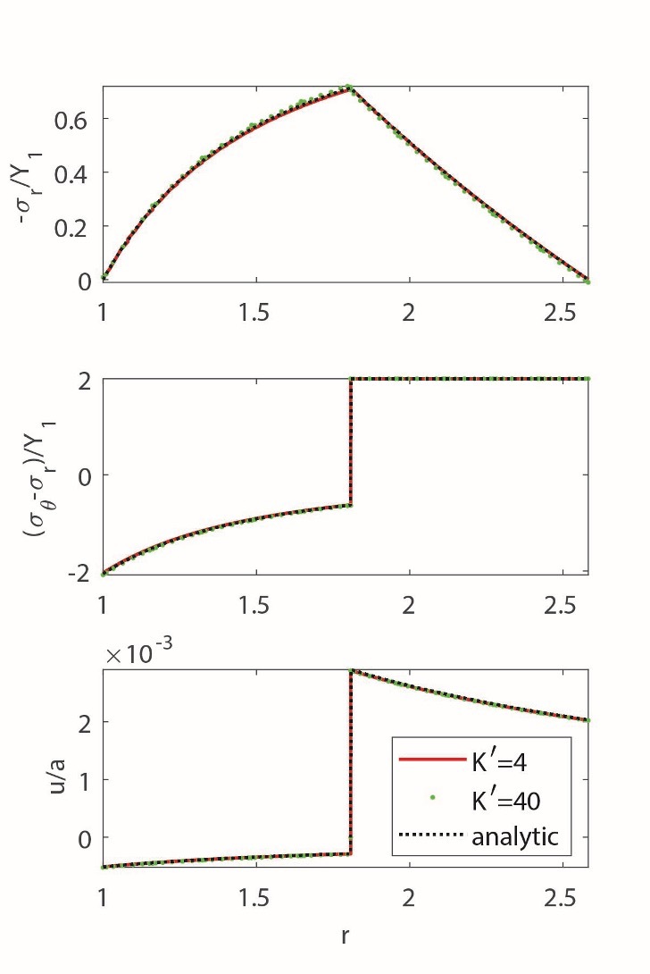
We replaced reaction radius, c, with reaction progress, ξ, using the equation. Figure 3 shows the obtained elastoplastic distribution of stresses and displacements in the REV under traction-free boundary conditions. The stresses in the REV are solely a result of the advancing reaction.

2.2.1. Effects of nonlinearity and comparison with the numerical solution

To evaluate the impact of nonlinearity, we compared the obtained analytical solution with the finite-strain numerical solution (fig. 3). Our numerical code incorporates an associative plastic flow rule with a von Mises yield criterion. Using a commonly adopted multiplicative approach, the strain gradient is decomposed into elastic and plastic components. For a more comprehensive understanding of the numerical implementation, further information can be found in the work by Moulas et al. (2023). Like in the previous elastic analysis, the influence of the nonlinear elastic parameter $K^{\mathstrut'}$ remains minor. The effect of plastic failure on the solution is more pronounced than nonlinear elastic effects. Our analytical solution was obtained assuming the entire nonreacted region experiences plastic flow. In the numerical solution, increasing load caused the gradual spreading of the plastic zone before reaching a fully plastic state. Comparison with the numerical solution shows that ignoring the gradual growth of the plastic zone in the analytical solution did not affect the result.

Figure 3.Comparison of elastoplastic stresses and displacements within REV: analytical vs. fully nonlinear numerical solutions corresponding to a reaction progress $ξ=0.4$. Simulations were performed at $\varphi = 0.15$, $\frac{\rho_{2}}{\rho_{1}} = 0.8$,$\frac{G_{2}}{G_{1}} = 0.7$, $\frac{K_{1}}{G_{1}} = 100$, $\frac{G_{1}}{Y_{1}} = 1500$.

2.3. Viscous and viscoplastic deformation of the rock

Viscous and viscoplastic solutions can be obtained quite similarly by replacing Hook’s law with linear viscous Newton’s law:

$$\frac{\partial v}{\partial r} - \frac{v}{r} = \frac{\sigma_{r} - \sigma_{\theta}}{2\mu}\mspace{6mu},\quad\frac{\partial v}{\partial r} + \frac{v}{r} = \frac{\sigma_{r} + \sigma_{\theta}}{2\eta} \tag{28}$$

Solution of equations together with the stress balance equation, condition at the reaction interface and boundary conditions give the following expressions for the velocities in the reacted and non-reacted zones for the purely viscous case:

$$v_{1} = - \frac{1}{2r\widehat{G}}\left( \frac{b^{2}}{b^{2} - a^{2}}A_{11}p_{e} + A_{12}p_{f} + A_{13}\frac{d\xi}{dt} \right) \tag{29}$$

$$v_{2} = - \frac{1}{2r\widehat{G}}\left( \frac{b^{2}}{b^{2} - a^{2}}A_{21}p_{e} + A_{22}p_{f} + A_{23}\frac{d\xi}{dt} \right) \tag{30}$$

The shorthand notations used in equations and are summarized in Appendix B. For the viscoplastic case, one has to add a yield criterion, obtaining the following velocities:

$$\begin{aligned} v_{1} &= \frac{\left( b^{2} - a^{2} \right)(1 - \Theta)}{2r}\frac{d\xi}{dt}\\ & \quad - \frac{a^{2}\Theta\left( a^{2} + \left( b^{2} - a^{2} \right)\xi \right)}{2\xi\left( b^{2} - a^{2} \right)r\mu_{2}}\\ & \quad \left( \chi Y_{1}\ln\frac{a^{2} + (b^{2} - a^{2})\xi}{b^{2}} + p_{e} \right) \end{aligned}\tag{31}$$

$$\begin{aligned} v_{2} &= - \frac{a^{2}\left( a^{2} + (b^{2} - a^{2})\xi \right)}{2\xi(b^{2} - a^{2})r\mu_{2}}\\ & \quad \left( \chi Y_{1}\ln\frac{a^{2} + (b^{2} - a^{2})\xi}{b^{2}} + p_{e} \right) \end{aligned}\tag{32}$$

2.4. Averaging

The previous relationships can be used to obtain expressions for the effective rheology of a porous, two-phase model. To derive macroscopic compaction equations for reacting materials, we substitute the obtained velocities given by equations and for the elastic case, and for the elastoplastic case, and for the viscous case, and for the viscoplastic case into the equations and . This results in the following elastic/elastoplastic compaction equations

$$\begin{aligned} \frac{d\varphi^{e}}{dt} &= - \frac{1}{K_{\varphi}}\frac{dp_{e}}{dt}\\ & \quad + \varphi\left( \frac{1}{K_{s}^{\mathstrut'}} - \frac{1}{K_{s}^{\mathstrut''}} \right)\frac{dp_{f}}{dt} - \kappa_{\varphi}\frac{d\xi}{dt} \end{aligned}\tag{33}$$

$$\frac{d\varepsilon^{e}}{dt} = - \frac{1}{K_{d}}\left( \frac{dp_{t}}{dt} - \alpha\frac{dp_{f}}{dt} \right) + \kappa_{d}\frac{d\xi}{dt} \tag{34}$$

Viscous/viscoplastic compaction equations take the following form:

$$\frac{d\varphi^{v}}{dt} = - \frac{p_{e}}{\eta_{\varphi}} - \kappa_{\varphi}\frac{d\xi}{dt} \tag{35}$$

$$\frac{d\varepsilon^{v}}{dt} = - \frac{p_{e}}{\eta_{d}} + \kappa_{d}\frac{d\xi}{dt} \tag{36}$$

Cases with and without plasticity will have different coefficients in the compaction equations, as summarized in tables 2–4. Combining both endmembers, we obtain the following macroscopic Maxwell-type viscoelastoplastic equations for reaction-induced volume change and porosity evolution:

$$\frac{d^{s}\varepsilon}{dt} = - \frac{1}{K_{d}}\left( \frac{d^{s}p_{t}}{dt} - \alpha\frac{d^{f}p_{f}}{dt} \right) - \frac{p_{e}}{\eta_{d}} + \kappa_{d}\frac{d^{s}\xi}{dt} \tag{37}$$

$$\begin{aligned} \frac{d^s \varphi}{d t} &=-\frac{1}{K_{\varphi}}\left(\frac{d^s p_t}{d t}-\frac{d^f p_f}{d t}\right)\\ & \quad +\varphi\left(\frac{1}{K_s^{\prime}}-\frac{1}{K_s^{\prime \prime}}\right) \frac{d^f p_f}{d t}-\frac{p_e}{\eta_{\varphi}}-\kappa_{\varphi} \frac{d^s \xi}{d t} \end{aligned}\tag{38}$$

In equations and , the reaction contributes to both porosity changes, as in classical dissolution-precipitation models, and solid volume change, as suggested by Malvoisin et al. (2021). In addition to explicit reactive terms in compaction equations, reactions also affect effective compressibility $K_{d}$, $K_{\varphi}$ and viscosity $\eta_{d}$, $\eta_{\varphi}$. Interestingly, the progressing reaction, in combination with the compressibility of the solid phase, leads to the appearance of two solid bulk moduli $K_{s}^{\mathstrut'}$ and $K_{s}^{\mathstrut''}$. These are usually attributed to the existence of a non-connected pore space (Detournay & Cheng, 1993). In our case, the difference between the two moduli results from the presence of a compressible solid phase with different mineralogical compositions and densities. Even when the bulk and shear moduli of mineralogical components are the same, these two moduli will still be different due to ongoing reaction and density differences. Effective bulk moduli and effective viscosities in equations and generally depend on porosity, reaction progress, density contrast, and material parameters of the constituents (tables 2–4). In the case of a reactive but incompressible solid, $K_{s}^{\mathstrut'} = K_{s}^{\mathstrut''}$. In the non-reacting limit with an incompressible solid, equations and reduce to compaction equations derived in (Yarushina & Podladchikov, 2015), which are shown to be consistent with Biot’s theory of poroelasticity (Biot, 1941) and Gassmann’s relations (Gassmann, 1951).

3. Properties of derived rheology

Solid compressibility, effective stress law, and independent set of equationsOur solution is obtained under the condition that immobile species are preserved in the system, i.e., that the following mass conservation equation holds:

$$\frac{\partial\left( \rho_{s}X_{s}(1 - \varphi) \right)}{\partial t} + \frac{\partial}{\partial x_{j}}\left( \rho_{s}X_{s}(1 - \varphi)v_{s}^{j} \right) = 0 \tag{39}$$

where X_s is the mass fraction of nonvolatile components in the solid. X_s is closely related to the reaction progress, ξ, defined earlier:

$$\xi = \frac{X_{s} - X_{s,initial}}{X_{s,final} - X_{s,initial}} = \frac{X_{s} - X_{s,initial}}{X_{s,eq}} \tag{40}$$

Both X_s and ξ can be calculated for each given reaction based on the molar masses of the compounds (see examples for various reactions in Appendix A). Mass conservation for immobile species can be combined with derived compaction equations and , leading to the very general form of the equation of state for a solid:

$$\begin{aligned} \frac{1}{\rho_{s}}\frac{d^{s}\rho_{s}}{dt} &= \frac{1}{K_{s}(1 - \varphi)}\left( \frac{d^{s}p_{t}}{dt} - \alpha^{\mathstrut'}\frac{d^{f}p_{f}}{dt} \right)\\ & \quad + \kappa_{s}\frac{d^{s}X_{s}}{dt} \end{aligned}\tag{41}$$

Here, solid bulk modulus K_s can be a complicated function of porosity, stress state, and reaction. Yet, it is related to the drained and pore bulk moduli through the relation familiar from non-reactive poroelasticity (Yarushina & Podladchikov, 2015)

$$\frac{1}{K_{s}} = \frac{1 - \varphi}{K_{d}} - \frac{1}{K_{\varphi}} \tag{42}$$

Changes in density due to reaction only are defined by the additional reaction expansion coefficient (see table 1 for notations)

$$\kappa_{s} = \frac{1}{1 - X_{s}} - \frac{\kappa_{d}}{X_{s,eq}} - \frac{\kappa_{\varphi}}{(1 - \varphi)X_{s,eq}} \tag{43}$$

The influence of fluid pressure on the density of the solid is given by the partitioning coefficient $\alpha^{\mathstrut'}$ that depends on the nature of the reaction as well as on porosity:

$$\alpha^{\mathstrut'} = \varphi\frac{G_{2}\Theta\xi(1 - \varphi) + (\Theta - 1)(K_{2} + G_{2})}{G_{2}\Theta\xi(1 - \varphi) + (\Theta - 1)(K_{2} + G_{2})\varphi} \tag{44}$$

When approaching the nonreactive limit, we recover the conventional relation $\alpha^{\mathstrut'} = \varphi$ (e.g., Yarushina & Podladchikov, 2015).

By incorporating the equation along with the equations provided in table 2, one can derive the following equation for the Biot-Willis parameter (Biot & Willis, 1957)

$$\alpha = 1 - \frac{1 - \alpha'}{1 - \varphi}\frac{K_{d}}{K_{s}} \tag{45}$$

that quantifies the partitioning of stress between the solid framework of the material and the pore fluid in the equation . The latter can be interpreted as an effective stress law for volumetric deformation. In the nonreactive limit $\alpha' = \varphi$, the equation reduces to the classical relation between elastic moduli and the equation to the classical elastic effective stress law. Note, however, that reaction progress generally depends on fluid pressure (Llana-Fúnez et al., 2012). Thus, the partitioning between the total stress and fluid pressure in the effective stress law for reactive systems can be modified even further.

Let us note at last that equations , and are linearly dependent. Thus, only two of them can be used simultaneously. Given that equations of state for various solids are well documented in thermodynamic databases such as Holland and Powell (1998) or Johnson et al. (1992), it is more convenient to use the equation and determine their parameters from databases for each given pressure, temperature, and reaction.

3.2. The relative importance of reactive terms

The dominance of either volume expansion or porosity reduction is contingent upon the relative significance of the reactive terms in equations and . In the absence of failure during the reaction, the ratio of effective reaction expansion coefficients can be determined by equations

$$\begin{aligned} \frac{\kappa_{d}}{\kappa_{\varphi}}_{(elastic)} &= \frac{G_{2}\xi}{\left( G_{1}(1 - \xi) + G_{2}\xi \right)\varphi},\\ \frac{\kappa_{d}}{\kappa_{\varphi}}_{(viscous)} &= \frac{\mu_{2}\xi}{\left( \mu_{1}(1 - \xi) + \mu_{2}\xi \right)\varphi} \end{aligned}\tag{46}$$

During the initial stages of the reaction, when $\xi \ll 1$, the volume expansion induced by the reaction is minimal, primarily leading to porosity reduction akin to dissolution/precipitation models. However, as the reaction progresses, the importance of volume expansion becomes comparable to porosity reduction. In materials with low porosity or when porosity becomes clogged due to the reaction, volume expansion is more important than porosity reduction, facilitating further accommodation of the reaction.

If inelastic failure or micro-cracking ahead of the reaction front is involved, the volume expansion and pore size reduction due to the reaction become equally important in both elastoplastic and viscoplastic cases, as given by the following ratios of reactive expansion coefficients

$$\begin{aligned} \frac{\kappa_{\varphi} - \varphi(1 - \varphi)(1 - \Theta)}{\kappa_{d} - (1 - \varphi)(1 - \Theta)}_{(elastoplastic)} &= \varphi - \frac{1}{\Theta},\\ \frac{\kappa_{d}}{\kappa_{\varphi}}_{(viscoplastic)} &= \frac{1}{\varphi} \end{aligned}\tag{47}$$

In low-porosity rocks, volumetric expansion due to reaction will be more pronounced than porosity reduction in viscoplastic rocks and of the same order of magnitude in elastoplastic rocks, as follows from the equation . If failure occurs in the reacted zone, then the influence of the reaction on the total volume will be minimal and result only in the porosity changes due to the reaction.

3.3. Dependence of failure limit on reaction

Failure criteria and can be used to evaluate the influence of chemical reactions on the material’s strength. The critical effective pressure required to start failure in the rate-independent elastoplastic case can be estimated as a minimum of $p_{c}^{1}$ and $p_{c}^{2}$ that are given below:

$$\begin{aligned} p_{c}^{1} &= \frac{G_{2}\xi(1 - \varphi)^{2}(1 - \Theta)}{\Theta\varphi\left( \xi + (1 - \xi)\varphi \right)}\xi\\ & \quad + \chi Y_{1}(1 - \varphi)\frac{G_{2}\xi + G_{1}\Theta\varphi(1 - \xi)}{G_{1}\Theta\varphi} \end{aligned}\tag{48}$$

$$\begin{aligned} p_{c}^{2} &= - \frac{G_{1}\xi(1 - \varphi)^{2}(1 - \Theta)(1 - \xi)}{\xi + (1 - \xi)\varphi}\xi \\ & \quad + \chi Y_{2}(1 - \varphi)\frac{G_{2}\xi + G_{1}\Theta\varphi(1 - \xi)}{G_{2}\left( \xi + (1 - \xi)\varphi \right)} \end{aligned}\tag{49}$$

Similarly, the failure limit in reacting viscoplastic rocks is given by a minimum of $p_{c}^{1}$ and $p_{c}^{2}$ that are given below:

$$\begin{aligned} p_{c}^{1} &= \frac{\xi\mu_{2}(1 - \varphi)^{2}(1 - \Theta)}{\Theta\varphi\left( \xi + (1 - \xi)\varphi \right)}\frac{d\xi}{dt}\\ & \quad + \chi Y_{1}(1 - \varphi)\frac{\mu_{2}\xi + (1 - \xi)\varphi\Theta\mu_{1}}{\mu_{1}\Theta\varphi} \end{aligned}\tag{50}$$

$$\begin{aligned} p_{c}^{2} &= - \frac{\mu_{1}(1 - \varphi)^{2}(1 - \Theta)(1 - \xi)}{\xi + (1 - \xi)\varphi}\frac{d\xi}{dt}\\ & \quad + \chi Y_{2}(1 - \varphi)\frac{\mu_{2}\xi + (1 - \xi)\varphi\Theta\mu_{1}}{\mu_{2}\left( \xi + (1 - \xi)\varphi \right)} \end{aligned}\tag{51}$$

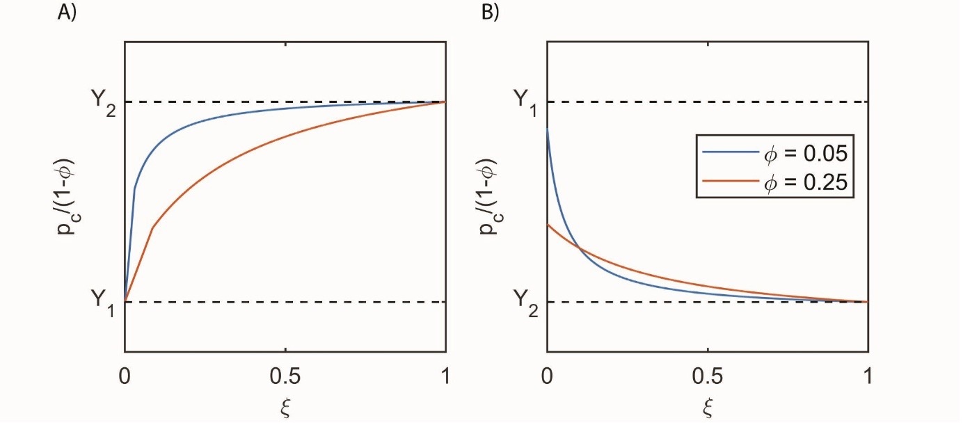
In the limiting cases of no reaction $\xi = 0$ and fully reacted material ($\xi = 1$), the usual limits for critical effective pressure $\left| p_{e} \right|_{\xi = 0} = Y_{1}(1 - \varphi)$ and $\left| p_{e} \right|_{\xi = 1} = Y_{2}(1 - \varphi)$ are recovered (Yarushina & Podladchikov, 2010, 2015). Figure 4 shows an example of the resulting critical pressure for viscous materials. Depending on whether the pristine material is weaker or stronger than the final reaction product, the material strength during the reaction will deteriorate or increase non-linearly. Experiments on exposure of Portland cement to CO₂-rich or H₂S-rich fluids indeed show an evolution of mechanical strength with reaction progress. Carbonated cement shows higher yield stress than unreacted cement (Lecampion et al., 2011), while cement exposed to H₂S loses its strength (Vrålstad et al., 2016). Cement weakening is associated with converting denser and harder iron to pyrite. In contrast, the conversion of portlandite into denser and harder calcite leads to the strengthening of cement.

Figure 4.Model predictions for failure limits in reactive viscous porous materials. (a) The reaction product is stronger than the pristine material, $\frac{Y_{2}}{Y_{1}} = 3$, $\frac{\mu_{2}}{\mu_{1}} = 2$ (b) The reaction product is weaker than the pristine material, $\frac{Y_{1}}{Y_{2}} = 3$, $\frac{\mu_{1}}{\mu_{2}} = 2$. Simulations were performed at $\frac{d\xi}{dt} = 10^{- 3}$, $\Theta = 0.8$ and two different values of porosity as indicated in the figure.

3.4. Implications for the “force” of crystallization

Our model predictions contribute to reconciling the varying estimates of the “force” of crystallization. It has long been recognized that chemical reactions involving an increase in the solid volume, or crystal growth, can generate stresses (e.g., Korenaga, 2025; Steiger, 2005; Weyl, 1959 and references therein). These stresses are often evaluated in terms of the “force” of crystallization, defined as the difference between the pressure on a growing crystal’s surface and the fluid pressure. Note that, as such, the “force” of crystallization has units of stress, not force. The thermodynamic models relate the “force” of crystallization to either the oversaturation of the solution phase (Correns & Steinborn, 1939) or the curvatures of the solid-liquid interface (Everett, 1961) and predict the “force” of crystallization that is on the order of several GPa (Wolterbeek et al., 2018). However, direct measurements of the “force” of crystallization generated during CaO hydration show stresses of up to 153 MPa, which constitute only 5% of the maximum value predicted by the thermodynamic theory for the “force” of crystallization (Van Noort et al., 2017; Wolterbeek et al., 2018). Similarly, experimental estimates for the “force” of crystallization during MgO hydration ranged from 20 to 200 MPa (Ostapenko, 1976). This mismatch can be attributed to the assumption of the ideal elastic behavior of a solid crystal in the previous models. As stresses reach the shear failure limit, which is on the order of several hundred MPa for many rocks, the inelastic processes will interfere with stress build-up. In our model, the “force” of crystallization can be estimated as the normal stress arising at the reaction front. It depends on the mechanical properties of the constituents, applied effective pressure, density change during the reaction, porosity, reaction kinetics, and the reaction progress:

$$F_{c}^{elastic} = \frac{dp_{e}}{\kappa_{c}^{e}} + \frac{G_{1}}{\kappa_{c}^{e}}\frac{(1 - \xi)(\Theta - 1)(1 - \varphi)^{2}}{\xi + (1 - \xi)\varphi}d\xi \tag{52}$$

$$F_{c}^{viscous} = \frac{p_{e}}{\kappa_{c}^{v}} + \frac{\mu_{1}}{\kappa_{c}^{v}}\frac{(1 - \xi)(\Theta - 1)(1 - \varphi)^{2}}{\xi + (1 - \xi)\varphi}\frac{d\xi}{dt} \tag{53}$$

Here,

$$\begin{aligned} \frac{1}{\kappa_{c}^{e}} &= \frac{G_{2}\xi}{G_{1}\Theta\varphi(1 - \xi) + G_{2}\xi},\\ \frac{1}{\kappa_{c}^{v}} &= \frac{\mu_{2}\xi}{\mu_{1}\Theta\varphi(1 - \xi) + \mu_{2}\xi} \end{aligned}\tag{54}$$

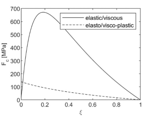
When plastic failure is not accounted for, the model may lead to high values of the “force” of crystallization for fast reactions (solid line in fig. 5). With the onset of shear failure, the “force” of crystallization is limited by the plastic flow. It depends on the applied external load, porosity, extent of reaction, and failure limit of the unreacted solid:

$$F_{c}^{plastic} = Y_{1}\ln\left( \xi + \varphi(1 - \xi) \right) + p_{e} \tag{55}$$

Its values are very close to the shear failure limit (dashed line in fig. 5). Given that the elastic, viscous, and plastic moduli and porosity depend on the curvatures of the solid-liquid interface and pore geometry and reaction progress, ξ, which is directly related to the supersaturation of the solution, our model is a generalization of both classical approaches by Correns and Steinborn (1939) and Everett (1961). Note, however, Mohr-Coulomb or Drucker-Prager failure criteria for rocks depend not only on the shear stress but also on the mean stress. Thus, under high lithostatic pressure, the failure criterion will be more difficult to reach, and thus, elastic or viscous estimates of the force of crystallization might be more relevant. This discussion is closely related to the broader debate surrounding tectonic overpressure—the phenomenon where pore pressures or localized stresses exceed lithostatic pressure in the Earth’s crust (Petrini & Podladchikov, 2000; Tajčmanová et al., 2014). Our model provides a framework for understanding how such overpressures might develop during mineral reactions that involve crystallization under confinement.

Figure 5.Model predictions for the “force” of crystallization in reacting elastic, viscous, elastoplastic, and viscoplastic porous media. For calculations, we assumed $\varphi = 0.25$, $\Theta = 1.2$, $G_{1} = 543\text{MPa}$, $\frac{G_{2}}{G_{1}} = \frac{\mu_{2}}{\mu_{1}} = 1.5$, $Y = 100\text{MPa}$, $\frac{d\xi/dt}{\mu_{1}} = 0.02$.

4. Closed system of equations for reactive transport in deformable media

The previous results can be used to derive a closed system of equations for reactive transport in deformable media. Consider a single chemical reaction in porous media saturated with a reactive fluid. Let us further assume that the solid phase consists of a nonvolatile component that remains in the solid and one or more volatile components that can easily be exchanged between the solid and fluid. We use its mass fraction to quantify the nonvolatile component in the solid phase $X_{s} = \frac{m_{nonvolatile}}{m_{solid}}$. The closed system of equations governing reactive transport in deformable porous rocks is summarized in table 5. It consists of three total momentum conservation equations (1)–(3), three fluid momentum conservation equations in the form of Darcy’s law, equations (4)–(6), the total mass conservation equation (7), and the mass conservation equation for the immobile species (8), as formulated by Malvoisin et al. (2017), Omlin et al. (2017), and Schmalholz et al. (2020).

When fluid consists of k components, concentration balance equations can be written for k-1 mobile species. A single balance equation must be formulated for a two-component fluid (such as a blend of H₂O and CO₂). It can be, e.g., the concentration of CO₂ with $C_{f} = \frac{m_{CO_{2}}}{m_{fluid}}$ and $C_{s} = \frac{m_{CO_{2}}}{m_{solid}}$, which changes due to chemical diffusion and advection (Beinlich et al., 2020; Vrijmoed & Podladchikov, 2022). Maxwell-type viscoelastic equations (10)–(15) given in table 5 can relate deviatoric stress and shear deformation. Porosity equation (16) can describe compaction. We still need fluid and solid equations of state and closure equations for chemical reactions. If the system is in local equilibrium, closure relations for chemical potential $\mu_{C_{f}}$, concentration of immobile solid $X_{s}$, and weight fraction of mobile components can be obtained from precalculated (lookup) tables. Given that fluid and solid can have quite complicated nonlinear equations of state depending on the temperature, pressure, and chemical composition, it is more convenient to use thermodynamic databases to recover those quantities as well (Beinlich et al., 2020; Vrijmoed & Podladchikov, 2022). Note that the commonly used mass exchange between fluid and solid (e.g., Rudge et al., 2011; Spiegelman et al., 2001) can be calculated from the mass balance equation for the solid instead of formulating explicit relations

$$\frac{1}{\rho_{s}}\frac{d^{s}\rho_{s}}{dt} - \frac{1}{1 - \varphi}\frac{d^{s}\varphi}{dt} + \nabla \cdot \mathbf{v}_{s} = \Gamma \tag{56}$$

5. Discussions and conclusions

A new micromechanical model for mineral replacement reactions and associated deformation is proposed. In contrast to previous models, where continuity of displacements is strictly enforced across the reaction front (Poluektov et al., 2018) or simply ignored at a risk of kinematic mismatch (Fletcher & Merino, 2001), we treat the reaction front as a sharp moving boundary with possible jumps in mechanical fields, analogous—mathematically—to second-order phase transitions, although not in the strict thermodynamic sense. We formulate the mass conservation law at the discontinuity. Stresses applied externally or generated during chemical reactions are accommodated by elastic, viscous, and plastic deformation. Obtained analytical solutions for deformation within the REV show good agreement with finite strain nonlinear numerical solutions.

An important outcome of the micromechanical model is the derivation of macroscopic (de)compaction equations that link changes in porosity and solid volume to stress, fluid pressure, and chemical reaction. Our results demonstrate that the interplay between reaction-induced deformation and stress can lead to a spectrum of behaviors: at one extreme, solid volume increase outpaces pore volume expansion, reducing porosity and potentially limiting fluid access and reaction progress; at the other, solid and pore volumes evolve in a balanced way that maintains fluid connectivity and allows the reaction to proceed toward completion. This continuum highlights the importance of capturing the relative rates of deformation in the solid and pore space when modeling reactive porous media.

Inelastic failure at the pore scale limits the unrealistically high build-up of the “force” of crystallization and favors the solid volume increase. In our model, the “force” of crystallization is on the order of the yield strength of the rock, which agrees well with experimental data. We show that chemical reactions lead to the appearance of two solid bulk moduli, which are usually attributed to the existence of a non-connected pore space (Detournay & Cheng, 1993). We formulate the effective stress law for the reactive porous rocks, which resembles the classical elastic effective stress law. However, the partitioning between the total stress and fluid pressure in the reactive systems is slightly altered. Our model predicts the dependence of effective bulk moduli, effective viscosities, and critical failure limits on porosity, reaction progress, density contrast, and material parameters of the constituents. To fully account for the coupling between reaction, deformation, and fluid flow, we derive a self-consistent macroscopic closed system of equations ready for implementation in numerical codes.

Acknowledgments

V.Y. acknowledges support from the ACT PERBAS project (No. 340832), funded through the Accelerating CCS Technologies (ACT) initiative. A.V. acknowledges financial support by the Russian Science Foundation (project 25-77-32001). We gratefully acknowledge Evangelos Moulas, Mark Brandon, and Reinier van Noort for their valuable comments and suggestions, which helped improve the quality and clarity of the manuscript. We also thank the anonymous reviewers for their constructive feedback.

Author Contributions

V.Y. has written the manuscript, derived analytical solutions, and performed numerical analysis. Y.P. contributed to the development of ideas. A.V. developed the algorithm and software for the numerical solution under finite strains.

Data Availability

The numerical code used in this study is available for download from https://zenodo.org/records/10021521

Editor: Mark Brandon, Associate Editor: Evangelos Moulas