A Physical Model for Accurate Paleotemperature Reconstruction From Fluid Inclusions in Halite

List of symbols

• a: fluid inclusion size, defined as the side length of the hypothetical cubic fluid inclusion.

• α: isobaric thermal expansion coefficient of the liquid phase (°C^-1).

• α_host: isobaric thermal volume expansion coefficient of the host crystal (°C^-1).

• β: haline contraction coefficient of the liquid phase (kgH₂O mol^-1).

• C: elastic compliance coefficient of the spherical cavity in the host, describing the volume change per unit of differential pressure ΔP (MPa^-1).

• γ: surface tension of the aqueous solution (N m^-1).

• g: gravitational acceleration (m² s^-1).

• G_host: shear modulus of the NaCl crystal along the <100> direction (MPa).

• h: depth of the water column (m).

• κ: isothermal compressibility coefficient of the liquid phase (MPa^-1).

• κ_host: isothermal compressibility coefficient of crystalline sodium chloride (MPa^-1).

• ℓ: the Berthelot-Laplace length (μm).

• ℳ_x: mass of compound x in the solution (kg).

• M_x: molar mass of compound x (kg mol^-1).

• m_NaCl,sat: NaCl saturation molality in the solution (mol kgH₂O^-1)

• m_x: molality of compound x in the solution (mol kgH₂O^-1).

• R_FI: radius of a sphere with a volume that equals that of the fluid inclusion (μm).

• ρ: density of the liquid phase (kg m^-3).

• ρ^∞: density of the vapor-saturated liquid phase at temperature T_h^∞ (kg m^-3).

• ρ_f: density of the liquid phase at entrapment conditions {T_f, P_f} (kg m^-3).

• ρ_host: density of solid sodium chloride (kg m^-3).

• P_ext: external pressure (MPa).

• P_f: fluid inclusion entrapment (= hydrostatic) pressure (MPa).

• P_L: pressure of the liquid phase (MPa).

• ΔP: differential pressure, or stress, on the fluid inclusion walls (= P_L – P_ext) (MPa).

• ΔP_lim: yield stress of the fluid inclusion; higher stress causes plastic deformation of the fluid inclusion walls (MPa).

• T: temperature (°C).

• T_f: formation temperature (°C); temperature of the brine at fluid inclusion entrapment.

• T_h,obs: observed liquid-vapor homogenization temperature (°C). Temperature at which the fluid inclusion transitions from a biphasic liquid-vapor state to a monophasic liquid state.

• T_h^∞: homogenization temperature of a hypothetical infinitely large system with flat vapor-liquid interface (°C).

• T_lim: temperature of FI yield point (°C).

• T_bin: temperature boundary between the stable and the metastable liquid-vapor state; also called “bubble binodal” (°C).

• T_sp: temperature boundary between the metastable and the mechanically unstable liquid-vapor state; also called “bubble spinodal” (°C).

• T_x: intersection point of two Brillouin shift - temperature curves measured in the monophasic liquid state and in biphasic liquid-vapor state of a fluid inclusion (°C). T_x = T_h^∞ within instrumental uncertainty.

• ΔT_L: Laplace pressure correction term (= T_h^∞ - T_h,obs) (°C).

• ΔT_P: hydrostatic pressure correction term (= T_f - T_h^∞) (°C).

• V: volume of the fluid inclusion (= a³) (m³).

• w_TDS: mass fraction of total dissolved salts.

• w_x: mass fraction of compound x in the solution.

1. Introduction

Fluid inclusions (FI) are microscopic volumes of fluid trapped in cavities within a host mineral. They are called “primary” if they were trapped during the formation of their host crystal, and here we call them “unaltered” if they have not undergone irreversible volume changes. For more than a century and a half, primary and (presumably) unaltered FI in minerals in magmatic/metamorphic rocks have been used as a paleothermometer (Roedder, 1984b; Sorby, 1858). Contrastingly, the paleothermometric potential of FI in surface and near-surface minerals has remained largely untapped. Halite (NaCl), in particular, is a common chemical sediment precipitated at the Earth’s surface, as it is composed of the two principal ions in seawater. Non-recrystallized, undeformed halite crystals containing primary FI are found in sedimentary basins from all Phanerozoic eras and beyond (Lowenstein et al., 2001; Weldeghebriel et al., 2022). The high solubility in water, 26.4 grams per 100 grams of solution at 25 °C and 0.1 MPa, accounts for extremely high sedimentation rates during periods of water deficit, for example, up to 0.1 m yr^-1 in the Dead Sea (Lensky et al., 2005). In turn, those high sedimentation rates generate sedimentary records at high temporal resolution, allowing seasonal (Brall et al., 2022; Sirota et al., 2017, 2021) and daily (Benison & Goldstein, 1999) environmental variations to be captured. Together with a purely physical temperature proxy — the density of the enclosed brine — halite FI represent ideal archives for paleoclimate research. Four major obstacles have hampered the use of halite FI for reconstructing Earth surface temperatures, and led some to dismiss halite FI paleothermometry altogether (e.g., Roedder, 1984a); nonetheless in the last 30 years all of these obstacles have been overcome.

1. Fluid inclusions in halite are typically single-phase liquid at room temperature and the absence of vapor bubble prevents measurements of liquid-vapor homogenization temperatures. Three techniques have overcome this limitation. With classical microthermometry spontaneous vapor bubble nucleation can be triggered by subjecting the inclusion to temperatures several tens of Celsius below T_h,obs (Roberts & Spencer, 1995); the large temperature excursion may, however, provoke irreversible deformation of the FI (Guillerm et al., 2020; Lowenstein et al., 1998). With the more recent technique of nucleation-assisted (NA) microthermometry, vapor bubble nucleation can be stimulated by means of single ultra-short laser pulses at temperatures only a few Celsius below T_h,obs (Krüger et al., 2007). With Brillouin thermometry, a temperature T_x can be determined by measuring the sound velocity first in the monophasic and then in the biphasic inclusion as a function of temperature with T_x representing the intersection of the two curves (El Mekki-Azouzi et al., 2015). Note, here the biphasic liquid-vapor state is accomplished by stretching the inclusions at temperatures far above T_x (Guillerm et al., 2020). The physical meaning of T_x is equivalent to the hypothetical temperature T_h^∞ at which homogenization of the inclusion into the liquid phase would occur without the effect of surface tension.

2. Halite is a very soft mineral (Mohs hardness 2.5) and may yield under the considerable deviatoric stress that builds up at the FI walls due to the pressure differential between the FI liquid phase and the host. Recently, the pressure differential causing plastic deformation of the halite FI walls, known as FI yield stress, has been quantified as a function of FI size, entrapment temperature and thermal history of the halite samples (Guillerm et al., 2020).

3. The surface tension at the FI liquid-vapor interface affects the temperature T_h,obs at which the vapor bubble collapses and the FI homogenizes to the liquid phase. To our knowledge, the first attempt to account for the effect of surface tension on homogenization temperature as a function of fluid inclusion size is due to Fall et al. (2009). More comprehensive models, including the effect of liquid compressibility, were later introduced, first for pure water (Marti et al., 2012), and then for any solution (Caupin, 2022). All these models assumed an isochoric (i.e., constant volume) fluid inclusion.

4. Complex concentrated brines have historically lacked accurate equations of state (EoS), required for assessing points (i), (ii) and (iii). The volumetric properties of multi-electrolyte brines are now well-constrained for the ranges of solute concentration, temperature, and pressure characteristic of halite FI (Al Ghafri et al., 2012, 2013).

The remaining challenges are to unify the aforementioned advances into a comprehensive model, and to incorporate in this model the interactions between the fluid and its halite host. Fluid-host interactions are expected to have a strong effect on the thermodynamic properties of halite FI in P_L-T-x space. This is because the solubility of halite in water (m_NaCl,sat) is highly dependent on temperature (T) and liquid pressure (P_L): for example in the NaCl-H₂O system at 25 °C and 0.1 MPa, $\left( \frac{\partial m_{\text{NaCl,sat}}}{\partial T} \right)_{P}$ and $\left( \frac{\partial m_{\text{NaCl,sat}}}{\partial P_{\text{L}}} \right)_{T}$ are 15 and 30 times higher, respectively, than the equivalent changes in quartz solubility in the SiO₂-H₂O system (Driesner & Heinrich, 2007; Morey et al., 1962); the temperature sensitivity of halite solubility is also highly dependent, and generally even greater, in aqueous solutions containing other salts in addition to NaCl. This is also because the coefficients of volumetric thermal expansion and isothermal compressibility of halite (α_host and κ_host) relative to those of the trapped liquid (α and κ) are significant: for example, in the NaCl-H₂O system, α/α_host = 26% and κ/κ_host = 14%, which is ~10 and 2 times the values for quartz, respectively (Kosinski et al., 1991; Levien et al., 1980). Last, the shear modulus (G) of halite along the <100> crystal direction is ~3 times smaller than that of quartz.

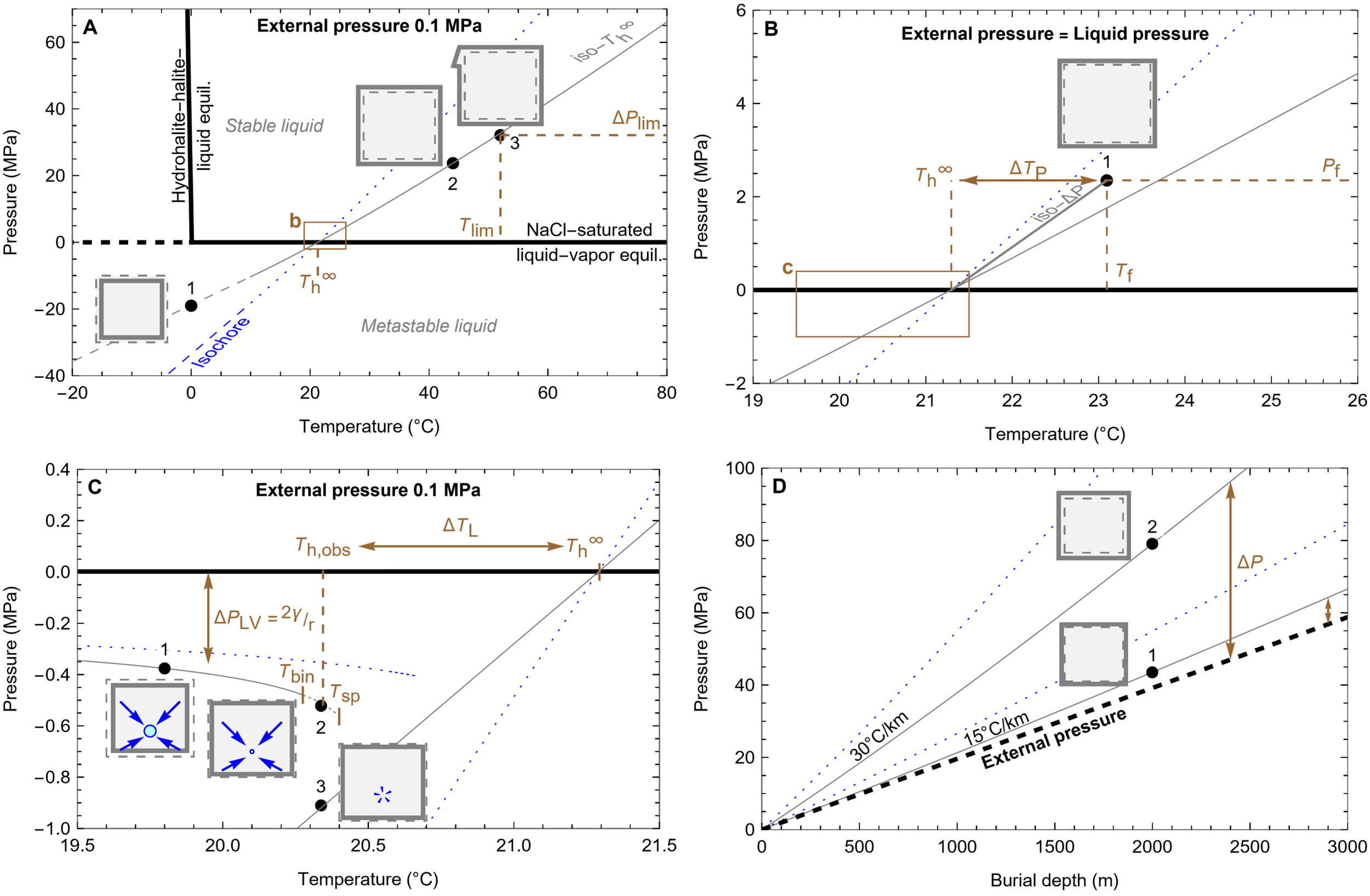
In this study, we develop HaliBubble, a comprehensive model for fluid inclusions in halite. We put the emphasis on using a robust EoS to describe the thermodynamic paths of the halite FI. Moreover, we acknowledge that the isochore assumption is not valid for halite FI, and therefore we focus on taking account of the substantial contributions of the host crystal to the volumetric and physico-chemical properties of the system. The model uses the “closed-system” assumption as mentioned by Roedder (1984b), that is, fluid inclusions experienced neither loss nor gain of entrapped water and solutes, except of sodium and chlorine through solubility reactions with the surrounding crystal. The main goal of HaliBubble is to predict the density, liquid pressure (P_L), yield point temperature (T_lim) and yield stress (ΔP_lim) of a halite FI, the effect of surface tension on T_h,obs, and the effect of entrapment (i.e., hydrostatic) pressure on T_h^∞.

2. Background and definitions

In the following, the subscript “f” indicates FI formation (= entrapment) conditions. The superscript “∞”, as introduced by Marti et al. (2012), refers to properties of the vapor-saturated liquid at temperature T_h^∞ and external pressure equal to atmospheric pressure (P_ext = P_atm, approximated to 0.1 MPa in this work), where T_h^∞ is the hypothetical homogenization temperature of a FI if surface tension did not provoke a premature collapse of the vapor bubble. The notation “{T, P_ext}” defines the external conditions of temperature and pressure (internal and external temperatures are considered always equal). We write the observed homogenization temperature T_h,obs to differentiate it from T_h^∞. Fluid inclusion size, a, is the side length of a hypothetical cubic FI. A halite FI is actually a parallelepiped with length a₁, width a₂ and depth a₃. Only a₁ and a₂ can be measured accurately under the microscope so we define a = (a₁a₂)^1/2, thereby assuming that a₃ = a.

2.1. Fluid inclusion saturation state

In this work, we assume halite FI are always saturated with respect to NaCl and thus located along the NaCl-saturated P_L-T plane in P_L-T-x space. This is justified by the rates of diffusion (J_D) and surface kinetics (J_S), which, for a change dT in temperature, follow:

$$\begin{array}{r} J_{\text{D}} = \frac{S}{V} \ k_{\text{D}} \ \left( \frac{\partial m_{\text{NaCl,sat}}}{\partial T} \right)_{P}, \\ J_{\text{S}} = \frac{S}{V} \ k_{\text{S}} \ \left( \frac{\partial m_{\text{NaCl,sat}}}{\partial T} \right)_{P}, \end{array} \tag{1}$$

where V = a³ and S = 6a² are the volume and surface area of a FI of size a; k_S is the surface kinetics rate constant of value 5 10^-4 m s^-1 (Alkattan et al., 1997); and k_D is the transport rate constant which, assuming a boundary layer thickness a/2, can be expressed 2D/a with D, the diffusion coefficient of NaCl in a NaCl-H₂O solution equal to 2.2 10^-9 m² s^-1 (for [NaCl] = 300 g/L and at 25 °C; Alkattan et al., 1997). Equation 1 can be integrated to obtain an exponential relaxation with time constants τ_D = V/(k_D S) and τ_S = V/(k_S S) for diffusion and surface kinetics, respectively. For a ranging between 10^-6 and 10^-4 m, we calculate that τ_D ranges between 38 μs and 0.37 s and τ_S ranges between 0.33 ms and 33 ms. The time needed to reach chemical equilibrium after a temperature (or pressure) change is thus lower than 1 s both in terms of diffusion and surface kinetics, so the halite FI can be considered always saturated with respect to NaCl.

2.2. Fluid inclusion liquid pressure

Fluid inclusions are commonly considered as closed isochoric systems of constant composition and thus the liquid pressure P_L in a monophasic FI is assumed to follow an isochoric trajectory with changing temperature. In halite FI, however, both the inclusion volume and the fluid composition undergo substantial changes with changing temperature, and thus the isochoric approximation is not applicable to describe the P_L-T properties of the system. Besides the thermal expansion and compressibility of the fluid — the only factors considered in the isochoric approximation —, HaliBubble incorporates the following additional factors (i)–(iii) with affected variables shown in brackets (volume V, mass ℳ_FI, density ρ) (fig. 1A):

1. thermal expansion/contraction of the host crystal [V, ρ];

2. elastic compliance of the cavity due to the pressure change [V, ρ];

3. dissolution/precipitation of NaCl at the solid-liquid interface due to the temperature- and pressure-dependent changes of the NaCl solubility [V, ℳ_FI, ρ].

Since the resulting thermodynamic path of the monophasic halite FI in P_L-T-x space intersects the NaCl-saturated liquid-vapor-equilibrium (LVE) curve at T_h^∞, we call it “iso-T_h^∞” curve, no longer implying that inclusion volume, fluid density, or composition are constant. The iso-T_h^∞ curve describes the reversible path of the liquid pressure P_L in the inclusion as a function of temperature when external pressure equals atmospheric pressure, as in the case under lab conditions. It is important to note that “iso-T_h” may have a different meaning in the literature: it may define the line that joins the conditions of FI liquid-vapor homogenization and of FI formation in the P-T space (Bodnar, 1994), which we here call “iso-ΔP” (see Section 2.5).

Figure 1.Halite FI in P_L-T-x space. A-C, NaCl-H₂O P_L-T diagram, sliced along the NaCl-saturated P_L-T surface in P_L-T-x space. Thermodynamic paths shown: phase equilibria (Parkhurst & Appelo, 2013; Valenti et al., 2012) (thick black lines), liquid phase of isochoric FI (blue dotted lines) and liquid phase of halite FI (gray lines). The isochoric FI has constant NaCl concentration (NaCl- and vapor-saturated at T_h^∞), so the P_L-T path is here projected on the NaCl-saturated P_L-T surface. Gray rectangles represent halite FI at temperature T (solid edges) vs. its initial shape at T_h^∞ (dashed edges) (volume change exaggerated). A, Liquid pressure in monophasic halite FI decreases (1) and increases (2) along the iso-T_h^∞ curve when T becomes lower and higher than T_h^∞, respectively. The slope of the iso-T_h^∞ is shallower than the isochore due to the contribution of host thermal expansion, elastic compliance and dissolution/precipitation. Beyond a pressure differential ΔP_lim that depends on FI size and that is reached at T_lim, the FI walls deform plastically (3) (here, FI size is 5 μm). Line dashing shows linear extrapolation. B, The difference between the hydrostatic pressure of entrapment (P_f) and the lab conditions (external pressure P_atm, fluid pressure P_vap at T_h^∞) results in T_h^∞ being lower than T_f by ΔT_P. The slope of the iso-ΔP curve is shallower than the isochore due to the contribution of host thermal expansion and dissolution/precipitation but steeper than the iso-T_h^∞ curve due to host compression and the absence of cavity elastic compliance. C, Surface tension at the vapor-liquid interface of the biphasic halite FI induces Laplace pressure (ΔP_LV), resulting in a stretched liquid (1). The liquid expands and the bubble shrinks as temperature increases, and the increasing curvature of the bubble further stretches the liquid (2). The bubble prematurely disappears at the temperature T_h,obs between the binodal and spinodal temperatures T_bin and T_sp and lower than T_h^∞ by ΔT_L (3) (here, FI size is 10 μm). The Laplace pressure is enhanced in the halite FI compared with the isochoric FI due to the contribution of host thermal expansion, cavity elastic compliance and dissolution/precipitation. Line dashing shows bubble metastability field. D, Liquid pressure in the monophasic halite FI as a function of sediment burial depth, for two different thermal gradients and a sediment density 2000 kg m^-3. The differential pressure (ΔP) between liquid and external pressures may be small or large depending on the thermal gradient.

2.3. Fluid inclusion yield stress

We define the differential pressure

$$\Delta P = P_{\text{L}} - P_{\text{ext}} \tag{2}$$

where P_L is the FI liquid pressure and P_ext is the external pressure (at the Earth’s surface, P_ext = P_atm). Positive and negative values of ΔP indicate compressive and tensile stress, respectively. For ΔP ≠ 0, the pressure P_L in the liquid is uniform but the stress on the host is anisotropic: the deviatoric stress is maximal at the liquid/host interface and decays away from the FI. The deviatoric stress at the liquid/host interface can be analytically calculated for a spherical FI in an isotropic host and equals 3/2 ΔP (Zhang, 1998). We define the “FI yield stress”, ΔP_lim, as the value of ΔP at which the deviatoric stress at the liquid/host interface equals the yield stress of halite. When ΔP ≤ ΔP_lim, the deviatoric stress generates a reversible, elastic strain. When ΔP > ΔP_lim, irreversible deformation of the host occurs at the vicinity of the FI (fig. 1A). This irreversible deformation is generally plastic for halite FI (Bodnar, 2003). Guillerm et al. (2020) quantified ΔP_lim as a function of FI size, assuming a spherical FI in an isotropic halite host (see formula in table 1). The knowledge of ΔP and FI size therefore allows calculation of the yield point temperature of the FI T_lim, which enables assessment of whether the FI have experienced plastic deformation during their geological history or after sample collection. In the case of plastic deformation, the information on T_f is lost.

Under sediment burial, P_ext is affected by geothermal gradient as well as lithostatic loading, itself a function of sediment density. These additional parameters become necessary considerations for the determination of sample history and risk of plastic deformation/damage to inclusions (fig. 1D).

2.4. Laplace pressure

The Laplace pressure (ΔP_LV) is a pressure differential between the vapor and the liquid phase. ΔP_LV arises from the surface tension at the interface between the vapor bubble and the liquid, and increases with increasing curvature of the interface, i.e., with decreasing vapor bubble radius, following the Young-Laplace relationship:

$$\Delta P_{\text{LV}} = 2 \ \frac{\gamma}{r} \tag{3}$$

with γ (N m^-1) the surface tension of the aqueous solution and r the vapor bubble radius (μm). The vapor in the bubble being at a pressure lower than vapor pressure at a flat surface according to the Kelvin equation, the liquid pressure is thus lower than vapor pressure at a flat surface and almost inevitably negative. In other words, the liquid in a biphasic vapor-liquid FI is under tension, or “stretched”. The Laplace pressure has two effects on the homogenization of the FI into the liquid phase (fig. 1C). First, the stretched liquid has a greater volume than the same liquid at the saturated vapor pressure P_vap (approximated to 0 MPa here); it would therefore fill the cavity, and the FI would thus homogenize, at a temperature lower than T_h^∞. Second, the biphasic liquid-vapor FI passes from a stable into a metastable state at the “binodal temperature” (T_bin), before the two-phase state finally becomes mechanically unstable at the “spinodal temperature” (T_sp), as defined by Marti et al. (2012). The existence of a metastable liquid-vapor state implies that the collapse of the vapor bubble, and thus T_h,obs, the temperature at which liquid-vapor homogenization is actually observed, is thermodynamically not clearly defined but may occur anywhere between T_bin and T_sp (T_bin ≤ T_h,obs ≤ T_sp < T_h^∞). Here we assume that the collapse of the vapor bubble occurs midway between these two temperatures: T_h,obs = (T_sp + T_bin)/2. We define the Laplace pressure correction term ΔT_L so that

$$T_{\text{h}}^{\infty} = T_{\text{h,obs}} + \Delta T_{\text{L}}. \tag{4}$$

2.5. Hydrostatic pressure

Halite FI form at hydrostatic pressure P_f that depends on depth of the overlying water column (P_f ≥ P_atm). P_f is the sum of the water and atmospheric pressures (in MPa) through:

$$P_{\text{f}} = 10^{- 6}\ \rho_{\text{f}} \ g \ h + P_{\text{atm}},\tag{5}$$

where ρ_f is the density of the brine (kg m^-3) at conditions {T_f, P_f}, g (m² s^-1) is the gravitational acceleration, and h (m) is the water column height. The surface-tension corrected homogenization temperature T_h^∞ of the FI occurs at a liquid pressure P_vap that is different from (and lower than) P_f. The volumetric and physico-chemical properties of the brine and host crystal vary as a function of pressure. It follows that the temperature of FI entrapment T_f at which the liquid fills the cavity when P_L = P_f is different from (and higher than) the temperature T_h^∞ at which the liquid fills the cavity when P_L = P_vap (fig. 1B). We define the hydrostatic pressure correction term ΔT_P as follows:

$$T_{\text{f}} = T_{\text{h}}^{\infty} + \Delta T_{\text{P}}.\tag{6}$$

The curve that joins conditions {T_h^∞, P_atm} and {T_f, P_f} in P_L-T-x space is different from the iso-T_h^∞; we call it the “iso-ΔP” curve. The iso-ΔP curve describes the reversible path of the liquid pressure P_L in the unaltered inclusion as a function of temperature when the liquid pressure P_L equals the external pressure P_ext. The iso-ΔP and iso-T_h^∞ curves are different for two reasons. First, formation conditions involve an external pressure P_f different from lab pressure P_atm and thus a compression-decompression of the host crystal, as opposed to the iso-T_h^∞ that is defined at P_atm and thus at constant host crystal volume. Second, the iso-ΔP curve involves a constant differential pressure (ΔP = 0) and therefore an absence of elastic compliance of the cavity, as opposed to the iso-T_h^∞ curve that involves P_L changing relative to a constant external pressure P_atm.

3. MODEL

HaliBubble applies to fluid inclusions in halite in the system Na-K-Mg-Ca-Cl-SO₄-HCO₃-H₂O. Any brine property mentioned in this section therefore refers to the property of a halite-saturated brine of complex chemical composition in the system Na-K-Mg-Ca-Cl-SO₄-HCO₃-H₂O, and thus not necessarily to the simple halite-saturated NaCl-H₂O case unless stated otherwise. Table 1 contains information on the liquid and solid EoS as well as on other parameters used in the model. HaliBubble uses the Al Ghafri et al. (2012, 2013) EoS for Na-K-Mg-Ca-Cl-SO₄-HCO₃-H₂O solutions. This EoS was fit by these authors on a single, hence internally consistent, density dataset. We chose the Al Ghafri EoS because it covers most of the range of temperature, pressure and concentration of interest to this work and for the internal consistency of the fit dataset. We tested the Al Ghafri EoS against volumetric data of several multi-electrolyte brines and found an accuracy of prediction of the thermal expansion and isothermal compressibility of brines better than ±3% (see Supplementary Information, SI). Note that the Al Ghafri EoS does not include Na₂CO₃; we found that using the NaHCO₃ EoS in place of the missing Na₂CO₃ EoS (at the same molar concentration) yielded adequate results.

3.1. Fluid inclusion liquid pressure (P_L)

In this section we develop the part of HaliBubble that calculates the liquid pressure P_L in a monophasic halite FI at external pressure P_atm.

3.1.1. Numerical expression

Let us first consider the deviation of the FI from the isochoric system due to the thermal expansion of the halite host. The density (ρ) of the liquid solution at temperature T and pressure P_L,1 is:

$$\rho_{1} = \frac{\rho^{\infty}}{ 1 + \alpha_{\text{host}} \ \left( T - T_{\text{h}}^{\infty} \right) }\tag{7}$$

where α_host is the thermal volume expansion coefficient of halite, ρ₁ is the density of the liquid brine at T and liquid pressure P_L,1, and the superscript “∞” refers to the brine conditions T_h^∞ and P_sat.

We can then add the elastic compliance of the cavity:

$$\rho_{2} = \frac{\rho_{1}}{1 + C \ \Delta P},\tag{8}$$

where C, the elastic compliance coefficient, is the relative volume change of the inclusion per unit of differential pressure ΔP (table 1), ΔP = (P_L,2 - P_ext) and P_L,2 is the liquid pressure after correcting the inclusion volume for elastic compliance.

To further account for the changes in NaCl solubility, we define

$$\rho_{3} = \frac{\mathcal{M}_{3}}{V_{3}}\tag{9}$$

where ℳ₃ (kg), V₃ (m³) and ρ₃ (kg m^-3) are the mass, volume and density of the FI when accounting for halite solubility in addition to host thermal expansion and cavity elastic compliance. From equation (9) we find (see SI)

$$\rho_{3} = \frac{\rho_{2} + \rho_{\text{host}} \ \left( R_{V} - 1 \right)}{R_{V}},\tag{10}$$

where ρ_host is the density of solid sodium chloride and R_V the volume ratio V₃ to V₂ expressed as

$$\begin{aligned} R_{V} &= 1 + \frac{\rho_{2}}{\rho_{\text{host}}}\\ & \quad \times \left( w_{\text{NaCL}} \ \frac{1 - w_{\text{TDS}}^{\infty}}{1 - w_{\text{TDS}}} - w_{\text{NaCL}}^{\infty} \right). \end{aligned}\tag{11}$$

w_NaCl and w_TDS are the mass fraction of solute NaCl and of all solute ions, respectively (for a NaCl-H₂O solution, w_NaCl = w_TDS). The superscript “∞” refers, again, to the brine conditions T_h^∞ and P_sat.

To calculate P_L as a function of T, T_h^∞ and the chemical composition of the FI, a numerical iteration scheme is applied that provides a solution for P_L with a precision better than 1%:

• first, we compute P_L,1 in equation (7) (1 iteration),

• then we compute P_L,2 in equation (8) (3 iterations),

• then we compute P_L,3 in equation (10) (1 iteration),

• finally, we compute P_L,2 in equation (8) again, this time using P_L,3 on the right hand side instead of P_L,1 (1 iteration).

The solution of the last iteration yields the sought-after liquid pressure P_L of a monophasic FI with given T_h^∞ at temperature T and external pressure P_atm and, if calculated across a temperature range, it defines the iso-T_h^∞ curve.

3.1.2. Analytical simplification

A simpler, analytical expression of the iso-T_h^∞ curve can be found in the vicinity of T_h^∞. Let us describe the amount of NaCl in the solution by the quantity

$$y = \frac{M_{\text{NaCL}} \ m_{\text{NaCL}}}{1\ + \sum_{i} \left( M_{i} \ m_{i} \right)}\tag{12}$$

where M_NaCl is the molar mass of NaCl (kg mol^-1) and m_NaCl the NaCl molality in the solution (mol kgH₂0^-1). M_i and m_i are the molar masses and molalities, respectively, of all other salt species i in the solution.

It can be demonstrated (see SI) that the slope of the iso-T_h^∞ curve in the vicinity of T_h^∞ follows:

$$\left( \frac{dP_{\text{L}}}{dT} \right)_{T_{\text{h}}^{\infty}} = \frac{\alpha + \lambda \ (\delta - \beta) - \alpha_{\text{host}}}{\kappa - \mu \ (\delta - \beta) + C},\tag{13}$$

where α, κ, β, λ and μ are temperature, pressure and concentration derivatives of brine quantities defined in table 2 and

$$\delta = \left( 1 - \frac{\rho}{\rho_{\text{host}}} \right) \ \frac{1}{1 + y}.\tag{14}$$

The analytical solution for (dP_L/dT)_Th^∞ (eq 13) can be used to calculate P_L:

$$P_{\mathrm{L}}=\int_{T_{\mathrm{h}}^{\infty}}^T\left(\frac{\mathrm{~d} P_{\mathrm{L}}}{\mathrm{~d} T}\right)_{T_{\mathrm{h}}^{\infty}} \mathrm{d} T\tag{15}$$

A comparison of the numerical and the simplified analytical model yields increasing deviations of P_L with increasing distance from T_h^∞. For multi-electrolyte brines listed in table 3 with T_h^∞ = 25 °C, average absolute deviations of P_L increase from 0.1 % for |T - T_h^∞| = 1 °C to 2.4 % for |T - T_h^∞| = 20 °C. The reason for the increasing deviations is the pressure-independence of the terms used in the analytical expression. The good match of P_L in the vicinity of T_h^∞, however, verifies that the model was properly constructed and implemented. In practice, we recommend to restrict the use of the analytical expression (eq 15) to a temperature range ± 25 °C around T_h^∞; within this range deviations from the numerical model are lower than ~3%, an uncertainty commensurate with the other uncertainties (see Section 4.4).

3.2. Laplace pressure correction term (ΔT_L)

Caupin (2022) developed the following analytical expressions for the spinodal and binodal temperatures (T_sp and T_bin, respectively) of the biphasic liquid-vapor state in an isochoric system:

$$T_{\mathrm{h}}^{\infty}-T_{\mathrm{sp}}=4\left(\frac{\ell}{R_{\mathrm{FI}}}\right)^{3 / 4}\left(\frac{\alpha}{1+\alpha T}\right)^{-1}\tag{16}$$

$$T_{\mathrm{h}}^{\infty}-T_{\mathrm{bin}}=2\left(3 \frac{\ell}{R_{\mathrm{FI}}}\right)^{3 / 4}\left(\frac{\alpha}{1+\alpha T}\right)^{-1}\tag{17}$$

where ℓ, the Berthelot-Laplace length, equaled 2/3 γ κ, R_FI is the radius of the sphere of equal volume than that of the FI (μm), γ is the surface tension at the liquid-gas interface of the vapor bubble (N m^-1), and T is temperature in °C. Here, to account for all temperature- and pressure-related density changes in the halite FI, we replace the thermal expansion coefficient α and the isothermal compressibility coefficient κ by the numerator and denominator of the right-hand side of equation (13), respectively:

$$\begin{aligned} T_{\mathrm{h}}^{\infty}-T_{\mathrm{sp}} &= 4\left(\frac{\ell}{R_{\mathrm{FI}}}\right)^{3 / 4}\\ & \quad \times \left(\frac{\alpha+\lambda(\delta-\beta)-\alpha_{\mathrm{host}}}{1+\left[\alpha+\lambda(\delta-\beta)-\alpha_{\mathrm{host}}\right] T}\right)^{-1} \end{aligned}\tag{18}$$

$$\begin{aligned} T_{\mathrm{h}}^{\infty}-T_{\mathrm{bin}} &= 2\left(3 \frac{\ell}{R_{\mathrm{FI}}}\right)^{3 / 4}\\ & \quad \times \left(\frac{\alpha+\lambda(\delta-\beta)-\alpha_{\mathrm{host}}}{1+\left[\alpha+\lambda(\delta-\beta)-\alpha_{\mathrm{host}}\right] T}\right)^{-1}, \end{aligned}\tag{19}$$

with

$$\mathcal{l} = \frac{2}{3} \ \gamma \ \left\lbrack \kappa - \mu \ (\delta - \beta) + C \right\rbrack.\tag{20}$$

As we defined T_h,obs = (T_sp + T_bin)/2, the Laplace pressure correction term becomes ΔT_L = T_h^∞ - T_h,obs.

3.3. Hydrostatic pressure correction term (ΔT_P)

3.3.1. Numerical expression

To put the density ρ^∞ of the monophasic halite FI at conditions {T_h^∞, P_atm} in relation to the original density ρ_f of the brine that was trapped at conditions at {T_f, P_f}, we need to take into account the following factors: the thermal expansion of the brine and of halite between T_h^∞ and T_f; the compression of the brine between P_vap and P_f; the compression of halite between P_atm and P_f; the cavity elastic compliance due to the pressure difference ΔP between the external atmospheric pressure P_atm and the saturated vapor pressure P_vap of the liquid at T_h^∞; and changes in solubility between conditions T_h^∞, P_vap and T_f, P_f. This can be expressed

$$\begin{aligned} \rho^{\infty} &= \frac{\rho_{\mathrm{f}}+\rho_{\text {host }}\left(R_V^{\infty}-1\right)}{R_V^{\infty}}\\ & \quad \times \left\{\begin{array}{l}\left[1-\alpha_{\text {host }}\left(T_{\mathrm{f}}-T_{\mathrm{h}}^{\infty}\right)\right]\\ \times \left[1+\kappa_{\text {host }}\left(P_{\mathrm{f}}-P_{\mathrm{atm}}\right)\right]\\ \times \left[1-C\left(P_{\mathrm{atm}}-P_{\text {vap }}\right)\right]\end{array}\right\}^{-1} \end{aligned}\tag{21}$$

with R_V^∞ , similar to equation (11), accounting for the volume change due to solubility change from conditions {T_f, P_f} to {T_h^∞, P_atm}:

$$\begin{aligned} R_{V}^{\infty} &= 1 + \frac{\rho^{\infty}}{\rho_{\text{host}}}\\ & \quad \times \left( w_{\text{NaCL}}^{\infty} \ \frac{1 - w_{\text{TDS,f}}}{1 - w_{\text{TDS}}^{\infty}} - w_{\text{NaCl,f}} \right). \end{aligned}\tag{22}$$

Solving equation (21) yields T_f, or ΔT_P = T_f - T_h^∞.

3.3.2. Analytical simplification

To develop an analytical expression of the hydrostatic pressure correction, we first break down the hydrostatic pressure correction term into a sum of its atmospheric and water components:

$$\Delta T_{\text{P}} = \Delta T_{\text{P,atm}} + \Delta T_{\text{P,water}}\tag{23}$$

with

$$\Delta T_{\text{P,atm}} = \frac{P_{\text{atm}}}{\left( \frac{dP_{\text{L}}}{dT} \right)_{T_{\text{h}}^{\infty}}}\tag{24}$$

$$\Delta T_{\mathrm{P}, \text { water }}=\int_{P_{\mathrm{atm}}}^{P_{\mathrm{f}}} \frac{1}{\left(\frac{\mathrm{~d} P_{\mathrm{L}}}{\mathrm{dT}}\right)_{\Delta P}} \mathrm{~d} P_{\mathrm{L}}\tag{25}$$

where (dP_L/dT)_Th^∞ is expressed in equation (13) and (dP_L/dT)_ΔP is the slope of the iso-ΔP curve along which the monophasic liquid halite FI has a constant ΔP = 0. As the iso-ΔP curve is different from the iso-_Th^∞ curve in that it involves host compression/decompression and no elastic compliance (see Section 2.5), its slope can be expressed by modifying the expression of the iso-T_h^∞ slope (eq 13) accordingly:

$$\left( \frac{dP_{\text{L}}}{dT} \right)_{\Delta P} = \frac{\alpha + \lambda \ (\delta - \beta) - \alpha_{\text{host}}}{\kappa - \mu \ (\delta - \beta) - \kappa_{\text{host}}}.\tag{26}$$

Equation (26) assumes temperature-independence of the terms of the equation. The analytical expression is therefore only valid when conditions {T_h^∞, P_atm} and {T_f, P_f} are close. We find that the difference between the numerical and analytical value of ΔT_P increases with water depth and virtually vanishes (~0.1%) for infinitely shallow waterbodies. On average for the brines listed in table 3 and for a T_h^∞ = 25 °C the difference is smaller than 0.1 °C for waterbodies shallower than 320 meters, with however a difference up to 0.5 °C for Paleo-Lake Gosiute. For deeper waterbodies and/or concentrations exceeding 0.5 mol kgH₂O^-1 of SO₄^2- or HCO₃^-, the use of the numerical expression is recommended.

3.4. Differential pressure during burial

Upon burial, a halite sample is subjected to elevated temperatures and pressures {T_b, P_b}. Under these conditions, there is a temperature T_b,eq at which a monophasic FI in the sample will have equal liquid and external pressures (P_L = P_b), in which case the FI walls are not subjected to deviatoric stress (ΔP = 0 MPa). For T_b < T_b,eq, ΔP < 0 so the FI walls are subjected to a tensile deviatoric stress; for T_b > T_b,eq, ΔP > 0 so the FI walls are subjected to a compressive deviatoric stress. We employ a two-step method to calculate ΔP under burial conditions. In a first step, we use a modified version of the hydrostatic pressure numerical expression (eqs. 21 and 22) (subscripts “b,eq” and “b” refer to conditions {T_b,eq, P_b} and {T_b, P_b}, respectively):

$$\begin{aligned} \rho^{\infty} &=\frac{\rho_{\mathrm{b}, \mathrm{eq}}+\rho_{\mathrm{host}}\left(R_V^{\infty}-1\right)}{R_V^{\infty}}\\ & \quad \times \left\{\begin{array}{l}\left[1-\alpha_{\text {host }}\left(T_{\mathrm{b}, \mathrm{eq}}-T_{\mathrm{h}}^{\infty}\right)\right]\\ \times \left[1+\kappa_{\text {host }}\left(P_{\mathrm{b}}-P_{\mathrm{atm}}\right)\right]\end{array}\right\}^{-1} \end{aligned}\tag{27}$$

where

$$\begin{aligned} R_{V}^{\infty} &= 1 + \frac{\rho^{\infty}}{\rho_{\text{host}}}\\ & \quad \times \left( w_{\text{NaCL}}^{\infty} \ \frac{1 - w_{\text{TDS,b,eq}}}{1 - w_{\text{TDS}}^{\infty}} - w_{\text{NaCl,b,eq}} \right). \end{aligned}\tag{28}$$

Equation 27 can be solved for T_b,eq. In a second step, we use a modified version of the FI liquid pressure numerical expression (eqs 7–11).

$$\begin{aligned} \rho_{\mathrm{b}} &= \frac{\rho_{\mathrm{b}, \mathrm{eq}}}{R_{\mathrm{V}}\left[1+\alpha_{\mathrm{host}}\left(T_{\mathrm{b}}-T_{\mathrm{b}, \mathrm{eq}}\right)\right][1+C \Delta P]}\\ & \quad + \left(\frac{\rho_{\mathrm{host}}\left(R_V-1\right)}{R_{\mathrm{V}}}\right) \end{aligned}\tag{29}$$

where

$$\begin{aligned} R_{V} &= 1 + \frac{\rho_{\text{b}}}{\rho_{\text{host}}}\\ & \quad \times \left( w_{\text{NaCL}} \ \frac{1 - w_{\text{TDS,b,eq}}}{1 - w_{\text{TDS}}} - w_{\text{NaCl,b,eq}} \right). \end{aligned}\tag{30}$$

We solve equation (29) for P_L using the same numerical scheme detailed in Section 3.1.1.

4. DISCUSSION

4.1. Model validation

In this section, we validate parts of HaliBubble against available empirical data.

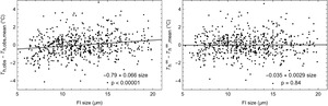
Calculation of the Laplace pressure correction term: As ΔT_L depends on the FI size, T_h,obs obtained from FI of equal density should display a positive trend as a function of size, and after applying the Laplace pressure correction the resulting T_h^∞ should no longer depend on inclusion size. To test the validity of the model we selected 860 FI smaller than 20 μm — our conservative estimate of FI yield stress size for these samples — from 28 halite samples analyzed with NA microthermometry by Arnuk et al. (2024). For each sample we calculated an average T_h,obs and then the difference of the individual T_h,obs values from the average. The same was done for T_h^∞. We find a significant T_h,obs-size linear trend of 0.066 °C/μm (p < 10^-5; fig. 2 and table 4) but no significant T_h^∞-size trend (p = 0.84), demonstrating the validity of the model.

Figure 2.T_h-size trend before and after Laplace pressure correction. T_h,obs and FI size data of 860 FI from 28 halite samples taken from Arnuk et al. (2024). See text for details.

Calculation of the hydrostatic pressure correction term: Brillouin thermometry measurements on a coarse halite crystal from the top of a drill core retrieved from the deepest lake floor of the Dead Sea yields an average T_x of 18.3 ± 0.9 °C (2 σ) (Guillerm et al., unpublished data). The sample grew on the lake floor under a 315 m-deep water column, during a period of permanent stratification in the early 1990s when the temperature of the hypolimnion remained annually stable at 22.2 ± 0.1 °C. We calculate ΔT_P = 3.8 °C for this sample, resulting in T_f = 22.1 ± 0.9 °C (2 σ), in excellent agreement with the monitored temperature (table 4).

4.2. Halite fluid inclusion: a non-isochoric system

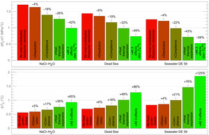
Halite FI are different from most other broadly studied FI in that their host readily interacts with the FI brine. We calculated the slope of the iso-_Th^∞ curve — (dP_L/dT)_Th^∞ — and the Laplace pressure correction term — ΔT_L — for three halite FI with different compositions (fig. 3) to illustrate the effect of fluid-host interactions on these parameters. We analyzed the deviation from the isochoric system individually for thermal expansion, elastic compliance and halite solubility to assess their relative contribution, as well as for the combination of the three processes. The combined effect is a reduction of (dP_L/dT)_Th^∞ by approximately half (-42% to -58% depending on composition) and a substantial increase of ΔT_L (+65% to +125% depending on composition). The thermal expansion of the halite host contributes the most to the deviation from the isochoric system, followed by cavity elastic compliance, and, last, halite solubility that has only a minor effect on (dP_L/dT)_Th^∞ and ΔT_L. We also observe that an increase of the concentration of other salt species in the NaCl saturated brine increases the effect of the host thermal expansion because the thermal expansion of the brine decreases. We note that the combined effect of the three processes on (dP_L/dT)_Th^∞ and ΔT_L is not simply the sum of the individual effects, because of interdependency: for instance, at a given temperature, the thermal contraction of the host reduces the volume of the cavity, thereby reducing the volume of the bubble, which further increases the Laplace pressure and the tension of the liquid, and therefore increases the elastic compliance of the cavity.

Figure 3.Contribution of dissolution, elastic compliance and thermal expansion of the host cavity to the liquid pressure P_L in the monophasic halite FI and to the Laplace pressure correction term ΔT_L. (dP_L/dT)_Th^∞ in the monophasic FI (Top) and ΔT_L (Bottom) are calculated in five different cases: (i) an isochoric FI; adding the contribution of the host cavity (ii) dissolution, (iii) thermal expansion or (iv) elastic compliance; (v) adding all three contributions. Calculations are made for T_h^∞ = 25 °C and for three different compositions (see compositions in table 3). ΔT_L is calculated for a 10 μm (1000 μm³) FI. Labeled percentage changes are calculated relative to the case of the isochore.

This work demonstrates that, counter-intuitively, reversible processes do affect the observed homogenization temperature of the inclusion (T_h,obs). In halite fluid inclusions, host crystal temperature- and pressure-induced volume changes, cavity elastic compliance and — to a lesser extent — solubility changes affect T_h,obs in two ways. First, they amplify the surface tension-induced premature collapse of the vapor bubble, resulting in a greater difference (ΔT_L) between T_h,obs and T_h^∞. Second, they decrease the slope of the iso-ΔP curve, which, if the FI was trapped at a pressure different from atmospheric pressure, results in a greater difference (ΔT_P) between T_h^∞ and T_f. These impacts of reversible processes on T_h,obs are reproducible: as long as the FI yield stress is not reached, successive measurements will give the same value of T_h,obs. But our work shows that reversible processes do affect T_h,obs in the sense that, for the same T_f, T_h,obs would be different if these reversible processes — host volume change, cavity compliance, FI wall dissolution/precipitation — did not exist. Also, the fact that the effect of solubility on T_h,obs is quite weak for the case tested here does not preclude a strong effect in other systems entailing a highly soluble host. Indeed, in the case tested here the increase of brine volume due to the addition of solute NaCl roughly keeps up with the cavity’s volume increase due to the FI wall dissolution, but that does not mean it will also be the case in other systems. The impact of reversible processes on microthermometric measurements was already mentioned, with a particular emphasis on halite for its high solubility and thermal expansion, by Yermakov (1965). However, Roedder (1984b) dismissed this issue, even for halite, stating that as long as volume changes are reversible the impact on microthermometric measurements must be null. This work supports the intuition of Yermakov and contradicts Roedder’s argument.

4.3. HaliBubble applications: illustration on Dead Sea halite sample

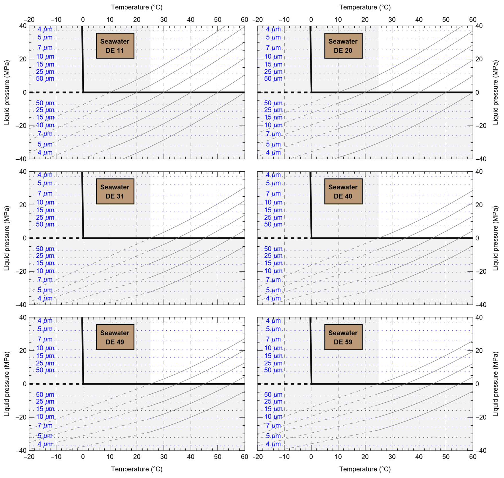
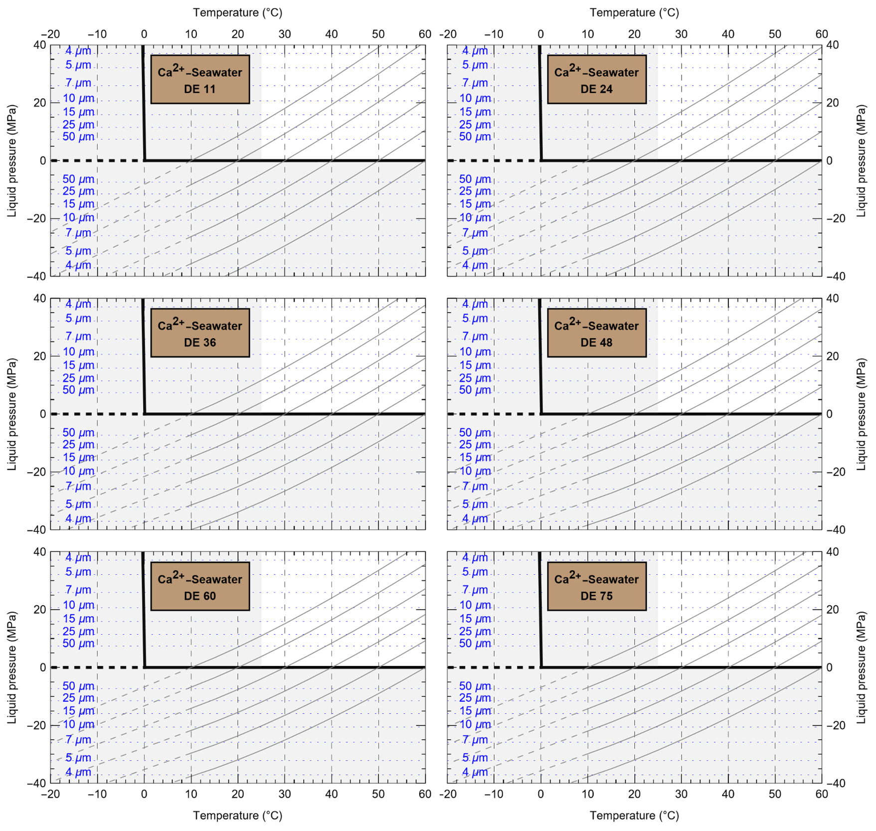
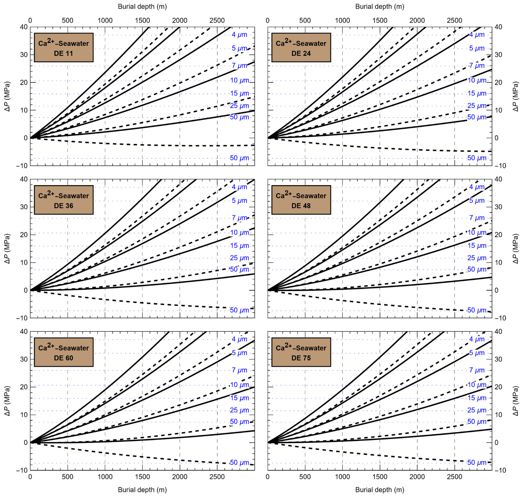
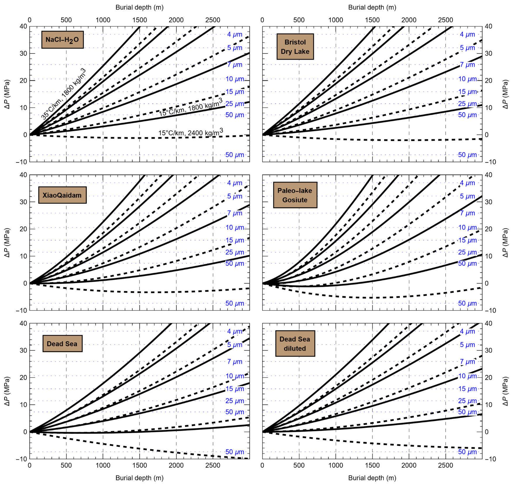
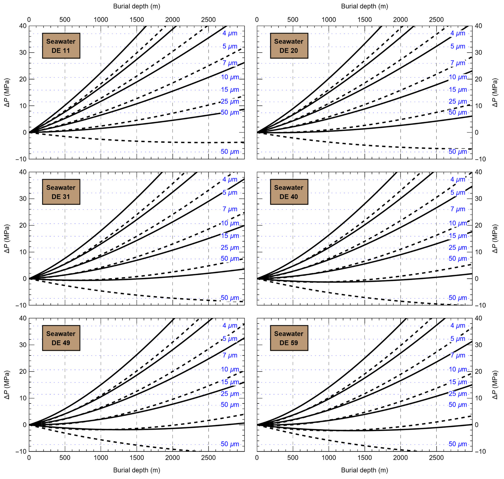
HaliBubble lays the foundation for improved paleotemperature reconstructions using halite FI. In the Appendix we show the following model results, for all the chemical compositions listed in table 3:

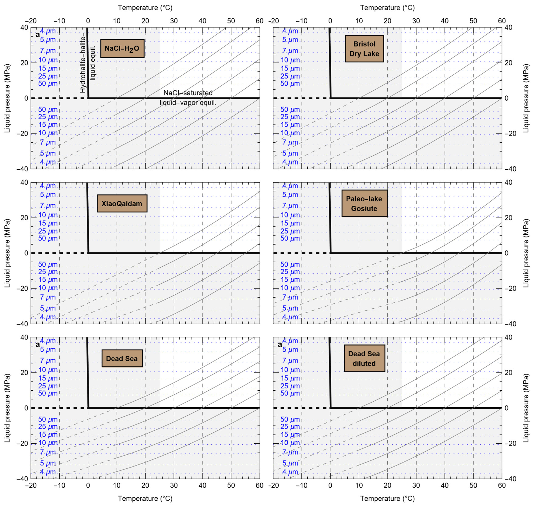
• iso-T_h^∞ curves for several T_h^∞ (fig. A1); and curves of ΔP as a function of burial depth for several geothermal and pressure gradients (fig. A2). These two types of curves are plotted along with ΔP_lim for different FI sizes and can be used to determine the maximum size of unaltered FI.

• ΔT_L as a function of FI size and T_h,obs (table A.1).

• ΔT_P as a function of water depth of sample formation and T_h^∞ (water and atmospheric components of ΔT_P in tables A.2 and A.3, respectively)

To further illustrate the applications of HaliBubble, in this section we describe the successive steps of paleotemperature analysis of a halite sample. The halite sample was collected 60 cm below the top of section 2-2 of core ICDP-5017-1-E from the deepest floor of the Dead Sea, in the southern Levant (Neugebauer et al., 2014). This sample comes from a shallow core depth (core composite depth: 5.93 m below lake floor) and thus formed only a few hundred years ago, therefore allowing the use of modern Dead Sea chemical composition (table 3) and water depth (330 m).

Selection of fluid inclusions: A preliminary determination of the maximum size of unaltered FI must be done before FI thermometry measurements, to avoid the measurement of FI whose volume changed irreversibly. It is done in two steps: by calculating the extremum ΔP undergone by the FI during burial and since core drilling. For both steps, we need to know T_h^∞. We do not know T_h^∞ of FI in advance, but based on air and water temperatures in the modern Dead Sea we use a first guess of T_h^∞ = 20 °C. A final determination of the maximum size of unaltered FI will be done after T_h^∞ is obtained to refine the selection of FI. First, we calculate the maximum ΔP during burial with the user interface (or fig. A2). With an average sediment density of 2000 kg m^-3, a geothermal gradient of 25 °C/km and a burial depth of 6 m, we find ΔP = 0.1 MPa; with such a weak differential pressure, we are certain that burial did not affect even the largest fluid inclusions. Second, we calculate the extrema ΔP since core recovery with the user interface (or fig. A1); for this we need to know the temperature extrema undergone by the core and sample. The minimum temperature undergone by the sample is very likely the storage temperature of 4 °C at the ICDP core storage facility. We estimate the maximum possible temperature undergone by the sample at 35 °C: the core drilling campaign took place in winter, daily air temperature maxima in winter in the Dead Sea are almost always lower than 30 °C, and we add 5 °C to take into account the potentially warmer temperature of surfaces exposed to the sun. Using these temperature estimates, we find that ΔP exceeded the yield stress ΔP_lim of FI larger than 34 μm. Note that, as a security measure, the user interface does not allow calculation of ΔP below the limit of natural extrapolation of the EoS, 10 °C, so here to roughly estimate it at 4 °C we proceeded as follows. We calculated ΔP at 10 °C (ΔP_10°C = -3.6 MPa) and at 11 °C (ΔP_11°C = -3.3 MPa), then deduced the slope of linear extrapolation of the iso-T_h^∞ (dΔP/dT_10°C ≈ [ΔP_11°C - ΔP_10°C]/1 °C = 0.3 MPa/°C), and finally calculated ΔP at 4 °C (ΔP_4°C = ΔP_10°C – 6 °C * dΔP/dT_10°C = -5.4 MPa).

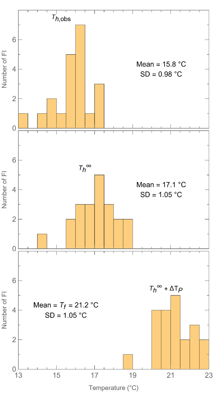
Experimental protocol: We measured the homogenization temperature T_h,obs of FI in the sample using NA-microthermometry at the University of Bergen (fig. 4). The protocol requires cooling the sample a few Celsius below T_h,obs (Arnuk et al., 2024) in order to be able to nucleate a vapor bubble in the FI with the femtosecond laser. We used a cooling temperature always above the minimum temperature experienced by the sample, 4 °C. We also made sure to never heat the sample above the maximum temperature experienced by the sample. This way, we did not alter FI smaller than the size threshold calculated above. If we had conducted Brillouin thermometry instead, we would have also made sure to conduct measurements within a narrow range of temperature, i.e., above 4 °C and well below 35 °C. Note that the protocol of classical microthermometry entails cooling samples to negative temperatures, generally -20 °C, in order to nucleate a vapor bubble in a large number of FI. Such low temperatures likely lead to plastic deformation of most FI, hence we recommend an overhaul of the protocol of classical microthermometry so that vapor bubbles are nucleated at a temperature as close to T_h^∞ as possible, even if it means obtaining less data.

Figure 4.Homogenization temperatures measured in a halite sample from the bottom of the Dead Sea and successive temperature corrections applied to obtain water paleotemperature (T_f). Mean and standard deviation (SD) are given in each subgraph.

Correction of Laplace pressure effect: The determination of T_h^∞ requires knowledge of ΔT_L, which is a function of T_h,obs, FI dimensions and chemical composition. We uploaded the input csv file containing this information in the user interface and obtained ΔT_L and T_h^∞ from the output csv file (fig. 4). The average T_h^∞ is 1.3 °C higher than the average T_h,obs (average FI size: 12.5 μm). We estimated again the FI size threshold with this new average T_h^∞ of 17.1 °C and found that FI smaller than 27 μm are unaltered.

Correction of hydrostatic pressure: The determination of water temperature during sample formation, T_f, requires knowledge of ΔT_P which is a function of chemical composition and water depth at the time. Water depths of ancient waterbodies are not necessarily known, in which case HaliBubble can be used to convert the water depth uncertainty into water temperature uncertainty. Here water depth is known (330 m) so we entered it in the input csv file and we could obtain ΔT_P in the output csv file. The histogram of water temperature is shown in fig. 4. We find T_f = 21.2 °C, close to the value of 21.7 °C monitored in the deep waters of the Dead Sea in 1959–1960 (Neev & Emery, 1967), thus suggesting little temperature variations in the region during the last few centuries. T_f is 5.4 °C greater than the mean T_h,obs, thus demonstrating the importance of using HaliBubble for accurate reconstructions of past environmental and climatic conditions. To give a sense of the paleoclimatic significance of such a bias correction, as a comparison the magnitude of global warming from the last Glacial Maximum to the following “warm” interglacial period of the Holocene is estimated at ~4 °C (Shakun et al., 2012).

Here it is worth mentioning that T_f = T_h^∞ + ΔT_P (eq 6) is an ideal conception only. In reality, a group of coeval unaltered primary halite FI formed at the same water depth and waterbody temperature will yield a range of T_h^∞ values with unimodal, Gaussian-like distribution and a standard deviation (SD) in the order of 1 °C (Arnuk et al., 2024). Arnuk et al. (2024) demonstrated that the temperature of the brine is well represented by (T_h^∞_avg + ΔT_P) where T_h^∞_avg is the average value derived from a group of coeval FI. Scatter of the T_h^∞ values occurs not only in halite FI but is also a characteristic feature of FI in other surface minerals such as stalagmites (Løland et al., 2022) and in magmatic and metamorphic minerals (Fall & Bodnar, 2018). The cause(s) of this scatter is/are currently unexplained and beyond the scope of this study. Possible factors of brine density variability upon FI entrapment, in a bulk solution of stable and constant temperature, include: disequilibrium (e.g., entrapment of a supersaturated brine), and thermal fluctuations along a brine/crystal interface due to a spatially heterogeneous crystal growth rate (crystal growth being, in general, an exothermic reaction).

4.4. Model limitations and uncertainties

A number of limitations and uncertainties should be considered when using HaliBubble.

Temperature extrapolation: The scarcity of empirical volumetric data of hypersaline brines below 25 °C (see SI) prevents direct testing of the natural extrapolation of the Al Ghafri EoS below 25 °C. Whereas pure water exhibits a density maximum, concentrated brines do not have this feature. Nevertheless, the slope of the density versus temperature becomes less negative at low temperature. Therefore, to estimate the reliability of the natural temperature extrapolation of the EoS below 25 °C, we compared the coefficient of thermal expansion of the brine (α) as calculated by linear versus natural extrapolation of the Al Ghafri EoS for the brine compositions listed in table 3. From 25 to 10 °C, deviations between the two extrapolations were below 5% for all brines, except for those with [SO₄^2-] or [HCO₃^-] > 0.5 mol kgH₂O^-1. We thus recommend natural extrapolation down to 10 °C. For sulfate or alkaline brines with [SO₄^2-] or [HCO₃^-] > 0.5 mol kgH₂O^-1, however, we do not recommend natural extrapolation at all. If one needs to correct for the effect of the Laplace or hydrostatic pressure below the extrapolation limit (10 or 25 °C depending on composition), we recommend the use of ΔT_P and ΔT_L at this extrapolation limit. If one needs to estimate P_L below the extrapolation limit, we recommend using linear extrapolation of the iso-T_h^∞ curve (as illustrated in Section 4.3).

Pressure extrapolation: The Al Ghafri EoS uses the Tammann-Tait equation for the pressure-dependence of density, allowing robust pressure extrapolation (Dymond & Malhotra, 1988). Applying the previous criterion of 5% deviation between natural and linear extrapolation to the compressibility coefficient, we find that natural pressure extrapolation is close to linear down to -100 MPa. We therefore recommend -100 MPa as a lower limit for natural extrapolation.

Concentration validity range: The Al Ghafri EoS is tested, and proved accurate, for highly concentrated chloride brines (ionic strength > 6 mol kgH₂O^-1) and less concentrated sulfate and alkaline brines (ionic strength < 6 mol kgH₂O^-1), with an uncertainty on the thermal expansion and isothermal compressibility of better than ±3% (see SI). According to equations 13, 18, 19, and 26, a 3% uncertainty on α and κ roughly converts into an uncertainty equal to, or slightly higher than, 0.03 °C per °C of temperature correction or 0.03 MPa per MPa of liquid pressure. There are presently no volumetric data available for NaCl-saturated brines that are highly concentrated in sulfate or (bi-)carbonate ions (⪆ 0.5 mol kgH₂O^-1), therefore HaliBubble may be inaccurate for these brine compositions. In particular, we find that highly alkaline brines, such as paleo-lake Gosiute brine, exhibit an exceptionally high temperature-dependence of their thermal expansion coefficient (α) (see paragraph Temperature extrapolation), which may indicate lower EoS accuracy for this specific chemical composition (i.e., an uncertainty on the thermal expansion significantly greater than 3%).

Spherical assumption: The halite FI is a parallelepiped with rounded vertices and edges. Because there is no analytical solution for such cavity geometry in terms of elastic compliance or yield point, we assume the halite FI is a sphere and consider that stress is applied on the (100) crystal faces. According to calculations of Zimmerman (1990), square sections exhibit a ~19% greater elastic compliance relative to circular sections. Assuming the cube-to-sphere elastic compliance ratio is the same as that of the square-to-circle, 1.19, a cubic FI is thus expected to have an elastic compliance 1.19 times greater than that of a sphere. This is an upper limit for halite FI given their rounded cube geometry. Given the contribution of elastic compliance to P_L and ΔT_L, ~20% (see fig. 3), we deduce that the spherical assumption is responsible for a maximum of 4% overestimation of P_L and ΔT_L in halite FI. Another simplification of the spherical model is that it assumes a uniform distribution of stress on the FI walls, whereas stress is greater along edges and vertices and smaller around face centers. Finite-element modeling of a 1:1:5 parallelepiped inclusion revealed a stress variation of ~10% between vertices and face centers (Mazzucchelli et al., 2018). As a result, the equation of Zhang (1998) (table 1) likely overestimates the halite FI yield point by ~5%. Note that if the spherical assumption leads to a 5% overestimate of ΔP_lim and a 4% overestimate of ΔP (or P_L), these two effects counterbalance so that the error on yield point temperature, T_lim, is only ~1% of |T_lim - T_h^∞|. Note that the deviation of the FI shape from a sphere has no consequence on the Laplace correction, because the vapor phase does not wet the FI walls, and the vapor bubble remains a sphere.

Total uncertainty: The main sources of uncertainty in HaliBubble are the effect of FI shape on elastic compliance as well as the coefficients of thermal expansion and compressibility of the brine. The uncertainty on elastic compliance is ~19%. The uncertainty on the coefficients of thermal expansion and compressibility is 3% for low-sulfate and low-alkalinity brines ([SO₄^2-] and [HCO₃^-] < 0.5 mol kgH₂O^-1) and unknown otherwise (see SI). On average for the low-sulfate and low-alkalinity halite FI chemical compositions listed in table 3, with T_h^∞ 25 °C and external pressure P_atm, by error propagation we find an uncertainty of 0.06 MPa/MPa on P_L and 0.07 °C/°C on ΔT_P. We find an uncertainty of 0.05 °C/°C on ΔT_L if FI dimensions are perfectly constrained. With a size uncertainty of 1 μm, the uncertainty on ΔT_L is 0.16 °C/°C, 0.09 °C/°C and 0.07 °C/°C for a 5, 10 and 20 μm FI, respectively. These relative uncertainties correspond to temperature uncertainties of 0.22 °C, 0.08 °C and 0.03 °C, respectively. For high-sulfate or high-alkalinity brines, the uncertainties are probably higher.

5. SUMMARY AND CONCLUSIONS

We developed a model for halite FI paleothermometry, H⁠a⁠l⁠iBubble, that takes into account the volumetric properties of the brine and its crystal host as well as chemical and mechanical interactions at the brine/host interface. H⁠a⁠l⁠iBubble provides the liquid pressure P_L in the monophasic inclusion, yield point temperature T_lim, Laplace pressure correction term ΔT_L and hydrostatic pressure correction term ΔT_P for various chemical compositions, pressure, temperature, and FI size. Application covers the chemical system Na-K-Mg-Ca-Cl-SO₄-HCO₃-H₂O, liquid pressure range -100 – 100 MPa, and temperature range 10 – 200 °C for low-sulfate low-alkalinity brines ([SO₄^2-] and [HCO₃^-] < 0.5 mol kgH₂O^-1) or 25 – 200 °C otherwise. HaliBubble is designed to be used in any halite FI paleothermometry study, regardless of technique – classical or NA microthermometry or Brillouin thermometry. It should be used for three purposes: (i) selecting unaltered FI based on their size and the temperature and burial history of the sample; (ii) correcting T_h,obs for premature collapse of the vapor bubble due to surface tension; and (iii) correcting for the weight of the water column. Processing a halite FI temperature dataset with these three steps will result in accurate paleotemperature estimates for the water in which halite formed, with uncertainties lower than 0.1 °C per °C of temperature correction and 0.1 MPa per MPa of liquid pressure in most cases. Tables and figures providing P_L vs. ΔP_lim, ΔT_L and ΔT_P for a selection of halite FI chemical compositions are found in the Appendix.

HaliBubble is an indispensable tool for accurate reconstructions of (paleo-)waterbody temperatures. Our calculations demonstrate that FI in halite cannot be considered as isochoric systems, that host-brine interactions within FI cannot be disregarded when measuring homogenization temperatures in halite FI, and that the Laplace and hydrostatic pressure correction terms are not negligible, amounting to several Celsius. The model reveals that proper documentation of the thermal history during collection, transport, storage and experimental handling of halite samples, and selection of FI based on their size and according to the documented thermal history, are essential practices to avoid potential artificially induced biases in the measured temperature data.

ACKNOWLEDGMENTS

EG thanks Robert B. Nachbar, Eric James Parfitt and Stephen Wolfram for their help in coding the user interface. We thank reviewers Robert J. Bodnar and Ronald J. Bakker for their valuable comments and suggestions that allowed a substantial improvement of the manuscript. We thank editor-in-chief Page Chamberlain and associate editor Daniel Ibarra for the efficient editorial process. This project has received funding from the European Union’s Horizon 2020 research and innovation programme under the Marie Skłodowska-Curie grant agreement No 101029939. Support from Agence Nationale de la Recherche is acknowledged by FC (grant no. ANR-19-CE30-0035-01) and VG (grant number ANR 22-CE01-0020-01). YK acknowledges funding from the European Research Council (grant no. 101001957). TKL acknowledges funding from the U.S.-Israel Binational Science Foundation Grant 2018/035 to TKL.

AUTHOR CONTRIBUTIONS

Emmanuel Guillerm: Writing – original draft, Visualization, Validation, Software, Resources, Investigation, Funding acquisition, Project administration, Formal analysis, Data curation, Conceptualization. Tim K. Lowenstein: Writing – review & editing, Validation, Resources, Funding acquisition, Project administration, Conceptualization. Véronique Gardien: Writing – review & editing, Validation, Resources, Funding acquisition, Formal analysis, Conceptualization. Achim Brauer: Writing – review & editing, Validation, Resources, Funding acquisition, Project administration, Formal analysis. Yves Krüger: Writing – review & editing, Validation, Investigation, Formal analysis, Data curation, Conceptualization. William D. Arnuk: Writing – review & editing, Validation, Software, Formal analysis, Data curation. Frédéric Caupin: Writing – review & editing, Validation, Software, Resources, Investigation, Funding acquisition, Formal analysis, Data curation, Conceptualization.

DATA AND SUPPLEMENTARY INFORMATION

A Supplementary Information (SI) file (Guillerm et al., 2025) is associated with this paper: https://doi.org/10.5880/GFZ.AVXH.2025.001. A cloud-based user interface of the model can be found at the following link: https://www.wolframcloud.com/obj/emmanuel.guillerm/HaliBubbleDataProcessing. The source codes of the model and of the user interface are written in Wolfram Language and can be found in the Wolfram Notebook Archive (model: https://notebookarchive.org/2025-01-b23umu8; user interface: https://notebookarchive.org/2025-01-b241xhv).

Conflict of interest

The Authors declare no conflict of interest.

Editor: C. Page Chamberlain, Associate Editor: Daniel E. Ibarra