Evidence for Low Dissolved Silica in mid-Mesozoic Oceans

1. INTRODUCTION

The global silicon cycle is closely linked to the carbon cycle and climate (e.g., Berner et al., 1983; Isson et al., 2022; Krissansen-Totton & Catling, 2020; Urey, 1952; Walker et al., 1981), but the record of marine dissolved silica concentration (DSi) through time is underconstrained. The silicon and carbon cycles are impacted by biotic processes, weathering, and global climate, and these cycles in turn influence climatic evolution over geologic time. However, constraining the global Si cycle, and particularly DSi, is difficult in deep time. During the Precambrian, mean oceanic DSi was likely supersaturated with respect to amorphous silica, and abiotic mineral precipitation was its primary sink (Maliva et al., 2005; Perry & Lefticariu, 2007; Siever et al., 1991). In contrast, mean DSi throughout the modern oceans is highly undersaturated due in large part to DSi drawdown by siliceous organisms, especially diatoms (Yool & Tyrrell, 2003). The timing and mechanism of the transition between the high DSi observed during the Precarmbrian and low DSi observed today is unclear. Filling this gap in understanding of the global Si cycle through time is important for establishing relationships between biological evolution, changes in past global climate, and major biogeochemical cycles. For example, high DSi could facilitate reverse weathering and thereby facilitate prolonged global warmth (e.g., Isson et al., 2022; Krissansen-Totton & Catling, 2020), while changes in productivity of biosilicifiers could explain episodes of cooling including via increases in rates of organic carbon burial in marine sediments (e.g., Katz et al., 2007; Pollock, 1997; Renaudie, 2016) and by changing reverse weathering dynamics (e.g., Dunlea et al., 2017). These interconnections between climate and coupled carbon-silica cycles take on added significance when considering the debated fate of diatoms in the face of present-day climate change (e.g., Taucher et al., 2022).

A key unresolved question is when DSi declined during the Phanerozoic and how this change related to the evolution and ecology of marine silica biomineralizers. A long-standing paradigm suggested that DSi remained elevated until diatoms radiated and dominated the marine silica cycle during the Paleogene (ca. 60 Ma) (Conley et al., 2017; Harper & Knoll, 1975; Maliva et al., 1989; Siever et al., 1991; Tréguer & De La Rocha, 2013). However, Fontorbe et al. (2016) and Fontorbe et al. (2017) found that during the Oligocene, Eocene, and Paleocene, DSi concentrations were already low and variable with depth and water mass age, indicating diatom uptake and dissolution and water mass age impacted—and led to low DSi—as early as 66 Ma. Mounting evidence points to lower DSi before the rise of diatom dominance on the marine Si cycle, including records suggesting low DSi from the Ordovician–Silurian (Trower et al., 2021) and during the Cambrian Explosion (Ye et al., 2021). Here, we address the following question: were mid-Mesozoic DSi concentrations similar to Precambrian DSi (> 500 μM) or more similar to modern DSi concentrations (<10 μM in surface ocean and ~70 μM in deep ocean)? If DSi in the mid-Mesozoic was more similar to the modern ocean, uptake by radiolarians and sponges was likely more important than canonically assumed. However, DSi during this time is poorly constrained. Moreover, more information is needed to understand the sensitivity of the Phanerozoic Si cycle to perturbation, including how changes in the utilization and concentration of DSi in the ocean may have affected marine ecosystems and vice versa (Harper & Knoll, 1975; Isson et al., 2022; Ritterbush et al., 2014, 2015).

The stable isotope ratio of silicon (δ³⁰Si) in sponge spicules reflects the DSi of water in which sponges grow, and is independent of depth, nutrient regime, and temperature (Hendry et al., 2010; Hendry & Robinson, 2012; Wille et al., 2010). The apparent silicon isotope fractionation (Δ³⁰Si = δ³⁰Si_sponge – δ³⁰Si_SW) between sponge spicules (δ³⁰Si_sponge) and seawater (δ³⁰Si_SW) is greater when DSi is higher, leading to a negative relationship between δ³⁰Si_sponge and DSi. On this basis, sponge spicule δ³⁰Si can be used to reconstruct DSi in deep time, assuming ancient sponges fractionate δ³⁰Si similarly to modern sponge taxa and provided δ³⁰Si_SW can be constrained. The assumption that modern fractionation processes during spicule formation can be extrapolated to the past is supported by the static nature of the sponge body plan across the Phanerozoic paleontological record (Suarez & Leys, 2022), the homology of silica biomineralization pathways across demosponges (Aguilar-Camacho et al., 2019), and the apparent poor adaption of silica utilization kinetics of both demosponges and hexactinellids to the relatively low DSi concentrations characterizing their modern habitats (Maldonado et al., 2020). In addition, culture experiments suggest the isotopic trend holds across different modern species (Cassarino et al., 2018), although with some dependence on spicule morphology (see Hendry et al., 2024 and discussion below). Together, these distinct sets of observations support the inference that little has changed in sponge silica biomineralization, or the associated concentration-dependent Si isotope fractionation, across the Phanerozoic.

An additional parameter needed to use sponge spicule δ³⁰Si to infer past DSi is the reconstruction of contemporaneous δ³⁰Si_SW. Radiolarians fractionate δ³⁰Si from seawater between –0.8‰ to –1.5‰ (Abelmann et al., 2015; Doering et al., 2021; Hendry et al., 2014), and radiolarian Δ³⁰Si values are not impacted by DSi. Thus, measuring δ³⁰Si in coeval radiolarians can help constrain δ³⁰Si_SW, and paired measurements of δ³⁰Si in sponge spicules and radiolarians can be used to infer DSi in the past (e.g., Fontorbe et al., 2016) and aid in building a better understanding of the coupled C and Si cycles and their role in global climate regulation (Fontorbe et al., 2020).

While the spicule DSi proxy has been applied over some intervals of geologic time, limited data have been presented from the Mesozoic and from intervals of major global environmental upheaval. Times of dramatic environmental change often have evidence for disruption to the global C and Si cycles, making them key events for increasing our understanding of these cycles through time. The Triassic–Jurassic boundary (TJB; 201.56 Ma; Wotzlaw et al., 2014) coincided with the eruption of the Central Atlantic magmatic province (CAMP; Marzoli et al., 1999), which emplaced massive amounts of basalt and emitted large amounts of CO₂ (e.g., Schaller et al., 2012; Steinthorsdottir et al., 2011) into the atmosphere–ocean system. This carbon release led to ocean acidification and warming, increased nutrient delivery, decreased oceanic oxygenation (e.g., Greene et al., 2012; Jost et al., 2017; Kasprak et al., 2015; Schoepfer et al., 2016; van de Schootbrugge et al., 2013), and ultimately the end-Triassic extinction (ETE) (e.g., Alroy, 2010). The eruption of CAMP is thought to have affected global weathering across the TJB, and sponge fossil evidence (Ritterbush et al., 2014, 2015) suggests a major perturbation of the marine silica cycle during the Late Triassic (Kidder & Erwin, 2001). During the early stages of marine recovery following the ETE, siliceous sponges dominated shallow marine benthic environments (Ritterbush et al., 2014, 2015); this ecological shift may have been enabled by the extinction of calcifying organisms and/or increased DSi delivery from enhanced weathering following CAMP CO₂ release and related climatic warming (Greene et al., 2012; Ritterbush et al., 2015). Therefore, constraining DSi across the TJB offers an opportunity both to 1) quantify DSi during the Mesozoic and 2) explore how the sponge spicule δ³⁰Si proxy can be used to test hypotheses about biological and environmental perturbations in the geological past.

2. SAMPLES AND METHODS

Sponge spicule δ³⁰Si values are typically measured on several (n ≈ 30) spicules from a single sediment or skeletal sample via multiple collector–inductively coupled plasma–mass spectrometry (MC–ICP–MS) (Hendry et al., 2010; Wille et al., 2010); however samples from 200 Ma are limited to lithified sedimentary rocks that host a small number of fully indurated spicules, which cannot be extracted from rock matrices without possible alteration and loss, and provide too few spicules for ICP–MS analysis. In this study, we used secondary ion mass spectrometry (SIMS), which allows analysis of individual spicules in complex matrices with analytical uncertainties of <0.3‰ on individual analyses (details in the supplemental information; also see Trower et al., 2021). We also measured modern spicules using SIMS to compare modern intra-spicule variability to that of ancient spicules.

2.1. Late Triassic–Early Jurassic stratigraphic sections and samples

We collected and screened samples from several stratigraphic sections spanning the Triassic–Jurassic boundary to identify material containing preserved sponge spicules suitable for stable Si isotope analysis by secondary ion mass spectrometry (SIMS). Samples from many sections that we investigated in thin section did not yield sufficient spicules of satisfactory quality for SIMS analysis. These included samples from St. Audrie’s Bay (UK; n ≈ 80), New York Canyon (Nevada, USA; n ≈ 50), the Lombardy Basin (Italy; n ≈ 200), and Csóvar (Hungary). Although we did observe sponge spicules in some of these samples, they were either no longer siliceous (e.g., replaced with carbonate) or so infrequent that the likelihood of intersecting them in a new thin section slice was very low, making them impractical to prepare for SIMS analysis. Further exploration of these stratigraphic sections or other locations may offer more spicule-yielding samples from this time interval. However, we did ultimately find suitable samples for analysis from sections near Levanto in northern Peru and Malpaso in central Peru.

The Levanto section (6°18’28"S, 77°53’04"W) comprises mudstones spanning the Late Triassic and Early Jurassic, as part of the Aramachay Formation of the Pucará group in the Peruvian Andes (fig. 1). High-resolution U–Pb dating and ammonite biostratigraphy from this section provide the Triassic–Jurassic boundary age (Guex et al., 2012; Schaltegger et al., 2008; Schoene et al., 2010; Wotzlaw et al., 2014), and previous work has reported carbon isotope stratigraphy and mercury contents and isotopes from the section (Yager et al., 2017, 2021). The section is relatively deep (well below storm wave base; speculatively ~500–1000 m) and the lithology changes little over the continuous four-million year section (fig. 1; Yager et al., 2017). Carbonate-rich mudstones host numerous carbonate-replaced radiolarians and rare siliceous spicules now preserved as quartz (fig. 2). We screened ~210 thin sections from Levanto (the same samples as those reported in Yager et al., 2017). We identified and analyzed four samples suitable for SIMS analyses that had >1% sponge spicules that were visibly well-preserved quartz. In addition to sponge spicules in the Levanto samples, we observed many radiolarians, most of which were characterized by calcite-replaced rims and silicified interiors (e.g., fig. 2B). We analyzed some radiolarians in an effort to constrain δ³⁰Si of seawater (δ³⁰Si_sw) during the Late Triassic and Early Jurassic. We used the published age model for this section (Yager et al., 2017) to place our δ³⁰Si in chronological context.

Figure 1.Simplified geologic map and correlated stratigraphic columns for samples discussed in this study. Extent of Pucará group and positions of the Levanto (northern Peru; Yager et al., 2017) and Malpaso (Central Peru; Ritterbush et al., 2015) sections are shown. Sample numbers denote stratigraphic locations. The two samples from the Malpaso section are Early Jurassic in age based on ammonite biostratigraphy (Ritterbush et al., 2015). Sections are very roughly correlated by the dashed line, as the only age constraints for the Malpaso section are the presence of the Sinemurian ammonites Arnioceras sp. 

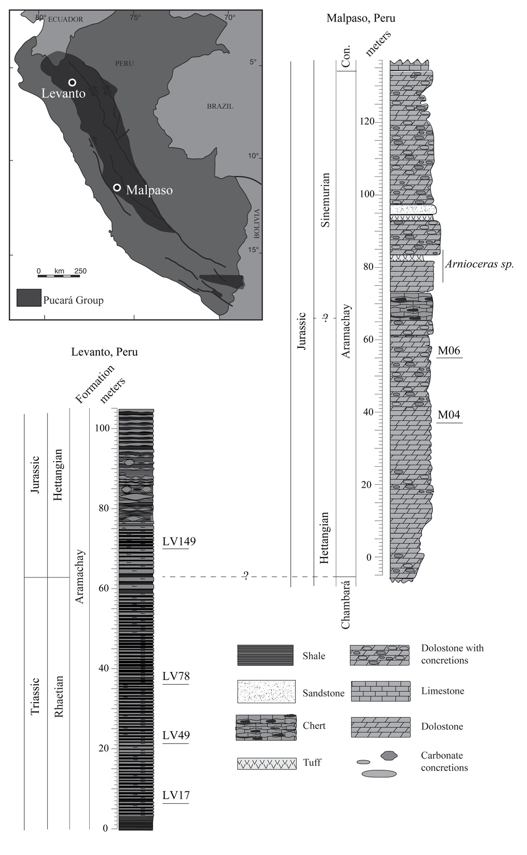
The Malpaso section (11°26’27"S, 75°59’03"W) is also part of the Andean Pucará group and contains a portion of the Late Triassic Chambará Formation and overlying Aramachay Formation. In contrast to the mudstones at Levanto, the Aramachay Formation at Malpaso is dominated by limestones. Arnioceras sp. ammonites in the Malpaso stratigraphic section (fig. 1; fig. 4 from Ritterbush et al., 2015) are Sinemurian, and while we lack more precise chronology, we speculate that the two Malpaso samples analyzed here which are below the ammonites are likely Early Jurassic (Sinemurian or Hettangian) in age.

Figure 2.Petrographic image examples of radiolarian and spicule preservation and δ³⁰Si_sponge analysis results for samples from the Levanto section. (A) Sample LV49F next to many radiolarians; note spicule 1 is seen also in (E). In this sample, radiolarians are dissolved and carbonate has precipitated within them, while the siliceous sponge spicule is quartz. (B) Cross polarized image of a radiolarian from sample LV23. Radiolarian test is siliceous and preserves some of the original structure; however, high porosity of the radiolarian may have hampered SIMS δ³⁰Si analysis when performed on similar radiolaria (this specific sample was not analyzed). (C, D) Photomicrographs of Levanto spicules with δ³⁰Si values; spicule mean ± 1SD in box. (E) LV49F spicule 1 with axial filament clearly visible.

2.2. Petrographic screening

We evaluated each sample petrographically and targeted SIMS analyses on spicules that were preserved as quartz and are distinct from their matrices (e.g., fig. 2). We screened each spicule and analysis spot for petrographic evidence of diagenetic alteration such as dissolution and reprecipitation and only report data from spicules that did not display petrographic evidence of replacement.

Samples from the Levanto section in many cases had samples containing quartz spicules. In contrast, petrography on samples from Malpaso indicated an extreme case of diagenetic resetting of spicule packstones and grainstones, and this site provides an obvious case of diagenetic alteration to compare to the better-preserved samples from Levanto. In one sample from Malpaso, spicules are composed entirely of calcite and their matrix is entirely quartz, indicating a complete dissolution and re-precipitation of carbonate and silicon during diagenesis; in another, while spicules are quartz, their boundaries are indistinct from their surrounding matrix and there is petrographic evidence of widening of the axial canal by dissolution followed by infill of secondary silica cement (fig. 3). We report results from the Malpaso samples, but given their diagenetic history do not consider them a reliable record of ambient DSi contents.

Sponge spicule morphology has recently been identified as a potential source of variation in δ³⁰Si values, with oxea spicules exhibiting lighter isotopic compositions than other spicule types in the same seawater conditions (Hendry et al., 2024). Here, given the paucity of quartz spicules available, we did not select spicules based on morphology. Most of the spicules we analyzed were monoaxial and relatively large while others were branching (e.g., figs. 2–3). Differences in the proportion of oxea spicules in our analyzed data could contribute to uncertainty in our record of changing DSi over time across the TJB, and further work focused on defined spicule morphology would be worthwhile, albeit challenging given the limited number of well-preserved spicules we were able to identify for analysis.

Figure 3.Petrographic image examples of spicule preservation and δ³⁰Si_sponge analyses from samples from the Malpaso section. (A, B) Malpaso sample MS3 in plane and cross-polarized light, respectively, with analyzed spicules outlined with white dotted line. Note chert spicule surrounded by chert matrix. (C, D) Plane and cross-polarized light images from sample M03 (not analyzed); note carbonate-replaced spicules surrounded by a silica-rich matrix.

2.3. Modern sponges

To test our analytical methods and to increase comparability to previous work on δ³⁰Si of sponges (primarily based on measurements made by MC–ICP–MS), we obtained spicules from four modern Hexactinellid sponges from the Natural History Museum of Los Angeles County (NHMLA) Invertebrate Collection and from one sponge found in a core from a cruise track from the Santa Monica Basin (Supplementary Table 1). Modern samples were subjected to the same workflow as fossilized samples, including petrographic analysis (fig. 4).

Figure 4.Modern sponge examples (A) Modern sponge spicule sample and (B) zoomed in view, with δ³⁰Si results; unheated sample mean ± 1SD in outlined box.

2.4. Analytical methods

Since siliceous sponge spicules were rare in investigated samples and were present in lithified matrix, we measured δ³⁰Si via secondary ion mass spectrometry (SIMS). Siliceous sponge spicules begin as opal and transform into quartz during diagenesis. We discuss the issue of possible matrix effects during SIMS analysis and preliminary heat treatment tests to address these effects during measurement of hydrated opal-A in modern sponges in the supplementary information (including Table 2).

2.4.1. Sample preparation

After screening thin sections for siliceous sponge spicules via petrographic observation, we cut new rock billets ~1 cm³ parallel to stratigraphy and bedding to maximize spicule surface area, and thus increase the opportunity for SIMS analyses and the chance to make multiple analyses within one spicule. Billets were mounted with silicon isotope standards (NBS28 and Caltech Rose Quartz) on the same one inch round thin section. We made whole thin section maps of each sample prior to SIMS analyses and identified siliceous spicules of interest. Modern sponges were cleaned and dissolved following established protocols (Hendry et al., 2010). Modern spicules were mounted with standard grains (NBS28) in SIMS thin section one inch rounds.

2.4.2. SIMS analysis of stable silicon isotope ratios

Silicon isotope analysis was carried out using a Cameca IMS 7f-GEO secondary ion mass spectrometer at the Microanalysis Center of Caltech. Data were collected over three sessions (November 2017, August 2018, and February 2019). A focused primary beam of –13 keV, ~5 nA, and 20–30 μm in size was used to sputter the sample surface, effectively encompassing the width of a spicule. Secondary ions (²⁸Si⁺ and ³⁰Si⁺) of +9 keV were collected with two Faraday Cups (FC) in the peak-jumping mode. The mass resolving power of the mass spectrometer was set at 3000, sufficient to completely resolve ³⁰Si⁺ from the ²⁹SiH⁺ interference. The counting rates of ²⁸Si⁺ of each spot varies between 5–7 × 10⁷ counts/s. The total measurement time for each spot was 8 minutes (including 60s pre-sputtering, secondary beam centering, mass calibration, and 20 cycles of data collection). In total, 282 total spot analyses were collected from quartz spicules from Levanto and 67 total analyses were collected from inferred biogenic sponge material (including spicules and matrix) from Malpaso. Sample measurements were bracketed by standard suites of the Caltech Rose Quartz and/or NBS28. The δ³⁰Si value was calculated for each sample by normalization to these standards (both defined as 0‰; δ³⁰Si = ((R_sample/R_standard)–1) × 1000).

2.4.3. Silicon isotope data reduction and screening

Raw ³⁰Si/²⁸Si ratio data within a single spot analysis that was >2SD from the mean of an analysis was removed for each analysis. δ³⁰Si values were calculated following Kita et al. (2009). All analyses with an analytical error >0.25‰ were removed. Results are reported in the supplementary data along with information about spicule preservation type and analysis quality.

Each SIMS spot (crater) was examined petrographically after analysis to see if there was a systematic difference in silicon isotope composition depending on the spicule preservation style or on the part of the spicule analyzed (e.g. intersecting an axial filament), and to ensure analyses were predominantly on the spicule. Each spicule was observed for preservation appearance (classified as “clear”, “brown”, “large”); overall, no systematic differences in δ³⁰Si were observed between spicule preservation types.

There is some indication that analyses falling off spicules tended to be more isotopically negative. However, in many cases what appeared to be off the spicule in plane polarized light looked like the analysis was on the spicule in reflected light. This difference is a product of the analysis and spicule geometry and the limitations of a thin section that is ~30 µm thick. Thus, we hesitate to make definitive evaluation of the effect of spot positioning but have eliminated obviously problematic individual analyses and rely on the large number of total analyses to average uncertainties associated with preservation, spot positioning, and intra-spicule variability. Removal of selected data in the screening process affects the average δ³⁰Si for each sample only slightly, well within the reported uncertainty.

2.5. Silicon isotope box model

To test plausibility of our results and their bearing on implied DSi (discussed in sections 3 and 4), we adapted the box modeling framework from prior work describing the Si isotope mass balance of the modern oceans (De La Rocha & Bickle, 2005; parameters used in this study in Supplementary Table 3). This model considers inputs and outputs from two boxes, representing the surface and deep ocean (fig. 5). Inputs are represented by a single term delivering dissolved silica to the surface ocean, encapsulating riverine, groundwater, and aeolian input fluxes. Outputs are in the form of biogenic silica (BSi) production and sedimentary deposition. We replace diatom production of biogenic silica (BSi), as implemented in the original model and later adaptations (Frings et al., 2016), with a combination of radiolarian and sponge BSi production, as thought to dominate the mid-Mesozoic oceans (fig. 6A). Since the location of most sponge BSi production in the past is difficult to constrain given the limited record of deep-sea sediments >180 Ma, we allow the proportion of sponge BSi production in the surface vs. deep ocean to vary as a tunable parameter in the model. Radiolarian BSi production occurs entirely in the surface ocean box, with dissolution and remineralization taking place during particle sinking.

Figure 5.Conceptual representation of the model used in this study, adapted from Frings et al. (2016) and De La Rocha and Bickle (2005). We replace diatom BSi production with radiolarian and sponge BSi production and use distinct representation of Si uptake to reflect different physiology of radiolarians and sponges (see main text Section 2).

We describe the evolution of the concentration of each Si isotope in the ocean, represented as [$XSi$] where x is either atomic mass 28 or 30, based on inputs and outputs from both the surface and deep ocean boxes for ³⁰Si and ²⁸Si separately. The surface ocean concentrations, ${XSi}_{surf}$, are described as:

$$\begin{align} \frac{d[30 \text{Si}]_{\text{surf}}}{dt} &= \bigg( F_{30 \text{Si, in, surf}} - B \text{Si}_{30 \text{Si, rad}} \\ &\quad - B \text{Si}_{30 \text{Si, sponge, surf}} - W_{\text{ex}} \cdot [30 \text{Si}]_{\text{surf}} \\ &\quad + W_{\text{ex}} \cdot [30 \text{Si}]_{\text{deep}} \bigg) / V_{\text{surf}} \end{align} \tag{1}$$

$$\begin{align} \frac{d[28 \text{Si}]_{\text{surf}}}{dt} &= \bigg( F_{28 \text{Si, in, surf}} - B \text{Si}_{28 \text{Si, rad}} \\ &\quad - B \text{Si}_{28 \text{Si, sponge, surf}} - W_{\text{ex}} \cdot [28 \text{Si}]_{\text{surf}} \\ &\quad + W_{\text{ex}} \cdot [28 \text{Si}]_{\text{deep}} \bigg) / V_{\text{surf}} \end{align} \tag{2}$$

and similarly, the equivalent concentrations in the deep ocean, ${XSi}_{deep}$, are described as:

$$\begin{align} \frac{d[30 \text{Si}]_{\text{surf}}}{dt} &= \bigg( F_{30 \text{Si, in, deep}} + \text{Diss}_{30 \text{Si, rad}} \\ &\quad - B \text{Si}_{30 \text{Si, sponge, deep}} + W_{\text{ex}} \cdot [30 \text{Si}]_{\text{surf}} \\ &\quad - W_{\text{ex}} \cdot [30 \text{Si}]_{\text{deep}} \bigg) / V_{\text{deep}} \end{align}\tag{3}$$

$$\begin{align} \frac{d[28 \text{Si}]_{\text{surf}}}{dt} &= \bigg( F_{28 \text{Si, in, deep}} + \text{Diss}_{28 \text{Si, rad}} \\ &\quad - B S i_{28 \text{Si, sponge, deep}} + W_{\text{ex}} \cdot [28 \text{Si}]_{\text{surf}} \\ &\quad - W_{\text{ex}} \cdot [28 \text{Si}]_{\text{deep}} \bigg) / V_{\text{deep}} \end{align}\tag{4}$$

where $F_{xSi,in,z}$ is the input flux of each isotope, ${BSi}_{xSi,y,z}$ is the consumption of each isotope by either radiolarians or sponges ($y$), $W_{ex}$ is the mixing flux of water between the surface and deep ocean, ${Diss}_{xSi,rad}$ is the release of each isotope by dissolution in the deep ocean, and $V_{surf}$ and $V_{deep}$ are the volumes of the surface and deep ocean, respectively (with $z$ reflecting either surface or deep).

The input fluxes, $F_{xSi,in,z}$, were determined based on compilation of Si fluxes to the oceans and associated isotopic composition (Frings et al., 2016), with input fluxes to the surface ocean comprising river ($F_{riv}$), groundwater ($F_{gw}$), and dust ($F_{dust}$) fluxes along with estuarine removal ($F_{est}$) and dissolution of river sediment ($F_{sed,\ diss}$), such that $F_{in,\ surf} = F_{riv} + \ F_{sed,\ diss} + \ F_{gw} + \ F_{dust}$. Input to the deep ocean comprises hydrothermal fluxes and alteration of oceanic crust. The flux for each isotope in equations (1)–(4) was determined based on the total Si flux to the oceans ($F_{in}$) and the isotopic value of that flux (${\delta^{30}Si}_{in}$), calculated as the weighted isotopic value of each input. Changes to the riverine flux (i.e., the weathering flux) thus change both the magnitude of the input flux as well as its net isotopic value.

Figure 6.Phanerozoic silica through time. (A) Relative importance of silica burial through the Phanerozoic (Kidder & Erwin, 2001) with δ³⁰Si_sponge from this and previous studies plotted against time binned into 10 Ma intervals (Cassarino et al., 2018; Fontorbe et al., 2016; Hendry et al., 2010, 2019; Hendry & Robinson, 2012; Trower et al., 2021; Wille et al., 2010). Data are plotted with median (white circle), 25^th/75^th percentiles (black box), data range without outliers (whiskers), and outliers as circles (outliers = >1.5x interquartile range). (B) Estimated DSi through time, with pink representing inferred DSi constrained by proxy records: (i) high DSi during the Precambrian (e.g., Conley et al., 2017; Siever et al., 1991); (ii) reduced DSi at the pre-Cambrian–Cambrian boundary based on first appearances of siliceous fossils (Siever et al., 1991); (iii) low DSi at the Ordovician–Silurian boundary (Trower et al., 2021); (iv) low DSi in the mid-Mesozoic (this study), and inferred to continue between ca. 200 and ca. 60 Ma; (v) Paleogene δ³⁰Si_sponge results that constrain DSi to low levels (Frings et al., 2016); (vi) modern DSi is between 10–180 μM.

We parameterize sponge consumption following Michaelis-Menten kinetics, such that:

$$\begin{aligned}{BSi}_{30Si,sponge}\ = \frac{ (V_{max,30Si} \cdot \ {\lbrack 30Si\rbrack}_{surf})}{(K_{m,30Si}\ + \ {\lbrack 30Si\rbrack}_{surf})}\end{aligned}\tag{5}$$

$$\begin{aligned}{BSi}_{28Si,sponge}\ = \frac{ (V_{max,28Si} \cdot \ {\lbrack 28Si\rbrack}_{surf})\ }{ (K_{m,28Si}\ + \ {\lbrack 28Si\rbrack}_{surf})}\end{aligned}\tag{6}$$

where $V_{\max}$ is the maximum uptake and $K_{m}$ is the half-saturation constant for each isotope. Following other studies modeling Si isotope fractionation in sponges, we adopt the same $K_{m}$ value for ³⁰Si and ²⁸Si given the same chemical behavior of the two isotopes, and thus the same transport mechanisms (Wille et al., 2010).

We estimate $V_{max,30Si}$ (uptake of the dominant Si isotope) based on the $V_{\max}$ observed in growth experiments for sponges ($V_{max,p}$, in μM Si h⁻¹ g⁻¹; Cassarino et al., 2018), the sponge stock per area on typical continental shelf area inhabited by sponge ($S_{sponge}$, g m^–2), and an estimate of the habitable area ($A_{sponge}$, m²), such that:

$$\begin{aligned} V_{max,30Si} \approx V_{max,p} \cdot S_{sponge} \cdot \alpha_{sponge}\end{aligned}\tag{7}$$

Sponge BSi production is partitioned between the surface and the deep ocean based on multiplying $V_{max,30Si}$ times the ratio $R_{sp}$, representing the proportion of total sponge production taking place in the surface. We relate $V_{max,28Si}$ to $V_{max,30Si}$ via the fractionation factor, $\alpha_{sponge}$, on the basis that the observed fractionation factor is defined by the ratio of rates of bio-silicification for the two isotopes. Therefore, isotopic fractionation is represented in the model by relating $V_{max,28Si}$ to $V_{max,30Si}$, as:

$$\begin{align*} V_{\text{max}, 28Si, \text{surf}} &= V_{\text{max}, 30Si, \text{surf}} \cdot \alpha_{\text{sponge}} \\& \cdot \frac{K_m + [28Si]_{\text{surf}}}{K_m + [30Si]_{\text{surf}}}\end{align*} \tag{8}$$

for the surface ocean, and analogously for the deep ocean. The fractionation factor $\alpha_{sponge}$ is determined as a function of dissolved Si concentration, following empirical calibration based on δ³⁰Si measured in sponge spicules and associated waters (Hendry et al., 2019):

$$\begin{align*} \alpha_{sponge,surf} &= 1 + \frac{ -4.71 + \frac{34.25}{8.29 + [30Si]_{surf} + [28Si]_{surf}}}{1000} \end{align*} \tag{9}$$

again with analogous representation for the deep ocean. The model could also be run with other parameterizations for $\alpha_{sponge}$, but we adopt this relationship as our purpose is to explore the general behavior of the model space (and we apply the same empirical calibration in Sections 3 and 4 when assessing DSi based on isotopic results). Total sponge BSi production (${BSi}_{sponge}$) in each box is calculated as the sum of ${BSi}_{30Si,sponge}$ and ${BSi}_{28Si,sponge}$, and the isotope ratio of sponge material by the ratio of these values. We treat the isotopic composition of sponge material in the surface ocean as representative of the material analyzed in our samples.

The uptake kinetics of silica by radiolaria are less well known than that for sponges, so we adopt a similar Michaelis-Menten description as used for sponges (as in eqs 5–6), noting the similar approach also used for diatoms in prior work (Frings et al., 2016). Lacking direct constraints on radiolarian physiology but considering the less competitive Si uptake by radiolarians relative to diatoms, we set the $K_{m}$ value for radiolarians to be the same as for sponges. We describe $V_{max,30Si}$ for radiolarians based on a parameter ($R_{rad–sponge}$) relating total radiolarian BSi production to total sponge BSi production, and we allow this parameter to vary. Similar to sponge uptake (following eq 8), we relate the radiolarian BSi production of ²⁸Si to the production of ³⁰Si via the fractionation factor $\alpha_{rad}$ which we assign a fixed value.

Radiolarian dissolution rate, $R_{diss}$, is described following Frings et al. (2016) based on kinetic parameters, as:

$$\begin{aligned}R_{diss} &= k_{diss}\ \\ & \quad \cdot (1\ – ({\lbrack 30Si\rbrack}_{surf} + {\lbrack 28Si\rbrack}_{surf})/C_{eq})\end{aligned}\tag{10}$$

where $k_{diss}$ is a dissolution rate constant, and $C_{eq}$ is the solubility of BSi in seawater. The total amount of dissolution in each box, ${Diss}_{rad}$, is calculated based on the dissolution rate, the production of BSi, and the time spent in the water column:

$$\begin{aligned}D{iss}_{rad,30Si,surf}\ =& \ R_{diss}\ \cdot \ {BSi}_{30Si,rad}\ \\& \cdot \ D_{surf}\ /\ v_{surf}\end{aligned}\tag{11}$$

$$\begin{aligned}D{iss}_{rad,28Si,surf}\ =& \ R_{diss}\ \cdot \ {BSi}_{28Si,rad}\ \\& \cdot \ D_{surf}\ /\ v_{surf}\end{aligned}\tag{12}$$

where D is the depth of the box (100 m for the surface and 5900 m for the deep) and v is the sinking velocity of particles. Analogous equations represent dissolution in the deep ocean.

The system of equations (1)–(4) was solved as a continuous set of differential equations using the Matlab function ode15s. This approach treats the oceanic Si cycle as a continuous process. In contrast, prior isotope box modeling built around this framework has calculated the mass balance in discrete timesteps, either by year (De La Rocha & Bickle, 2005) or 1/32 of a year (Frings et al., 2016), allowing Si to accumulate in each time step and then be drawn down by BSi production, with net isotopic fractionation during drawdown described as a Rayleigh process. The dependence of $\alpha_{sponge}$ on dissolved Si concentration violates the assumption of constant fractionation that is inherent to the Rayleigh model, and the multiple competing pathways of Si uptake (i.e., both sponges and radiolarians in the surface ocean box) add complexity. Treating the problem as a continuous process allows for explicitly representing the balance of each isotope based on the fractionation factors for sponges and radiolarians.

3. RESULTS

We report 238 δ³⁰Si values from 76 spicules from four Levanto samples and 54 values from spicules and matrix from two Malpaso samples (fig.7; Supplementary data tables 4–6). We report our modern silicon isotope results in Supplementary figure 7. Analytical uncertainty was ~0.5‰ (1 s.d.) based on reproducibility of standards (NBS28 and Caltech Rose Quartz). The δ³⁰Si values from the four Levanto section samples increase throughout the studied interval, with sample mean δ³⁰Si values and 1 s.d. of –0.98 ± 0.91‰ (samples from 203.89 Ma), –1.27 ± 0.33‰ (202.83 Ma), –0.25 ± 0.55‰ (202.09 Ma), and 0.46 ± 0.64‰ (sample from 200.88 Ma). The mean δ³⁰Si ± 1 s.d. of late Triassic analyses (all those >201 Ma) was –0.34 ± 0.90‰.

Our use of SIMS also provides information about variability in δ³⁰Si within individual sponge spicules. The Mesozoic spicules in this study preserve intra-spicule variability in δ³⁰Si on the same scale as modern δ³⁰Si, which we interpret as suggesting whole-spicule dissolution and precipitation from fluid did not occur. Individual spicules in each sample also differ from one another in terms of mean δ³⁰Si value, which may be consistent with preservation of primary values rather than homogenization during diagenesis (discussed further in section 4.1). Multiple spicules in one sample likely preserve a range of temporal and individual sponge information, and we interpret them as reflecting a characteristic δ³⁰Si value for the region and not a specific depth. We therefore view the average values of all analyzed spicules as a representative average of their given time interval.

Figure 7.Sponge silicon isotope results. δ³⁰Si_sponge values from Levanto (using age model from Yager et al., 2017), Malpaso, and modern samples from this and previous studies. Sample averages are plotted (where applicable) with 1 SD.

Radiolarian δ³⁰Si analyses from the Levanto samples yielded highly variable δ³⁰Si values. Radiolarians in our samples had extremely variable preservation, low ion counts via SIMS, and highly variable δ³⁰Si values. We therefore deemed the radiolarian δ³⁰Si data we collected to be unreliable records of primary δ³⁰Si values. Trower et al. (2021) found similarly dubious δ³⁰Si results for radiolarians from Paleozoic rocks, in which silicified interiors of radiolarians were unlikely to represent their primary value. We therefore used previously reported radiolarian δ³⁰Si data from Bôle et al. (2020) and Bôle et al. (2022) to constrain δ³⁰Si_sw from coeval sections.

Bôle et al. (2020) and Bôle et al. (2022) measured and reported radiolarian δ³⁰Si from the Inuyama and Katsuyama sections of Japan, respectively. Their data span the Late Triassic and Early Jurassic, providing a potential constraint on δ³⁰Si_SW during this time. These records comprise distal pelagic cherts where up to 90% of the matrix is siliceous; the authors use a mass-balance approach to estimate the likelihood of isotopic resetting during diagenesis and conclude their overall data is not primarily diagenetic. These radiolarians are presumed to record surface ocean δ³⁰Si_SW. Radiolarian data of Bôle et al. (2020) had an average value of 1.3 ± 0.3‰; data from Bôle et al. (2022) that hit radiolarian molds precisely had an average value of 1.2‰. Based on the fractionation radiolarians typically exhibit from seawater and these average values, we estimate a δ³⁰Si_SW of 2.7‰ at the time, though we note that seawater isotopic composition may have evolved over time between the Late Triassic and Early Jurassic and that we are unable to constrain any differences due to depth or location.

Considering our average end-Triassic sponge spicule δ³⁰Si values from Levanto, seawater δ³⁰Si_SW of 2.7‰ based on the radiolarians from Japan, and the modern DSi-δ³⁰Si_sponge calibration, our results indicate end-Triassic DSi was between 20 and 100 µM (fig. 8). This range takes into consideration different species-dependent isotope effects observed across different sponges (Cassarino et al., 2018). We also note that Hendry et al. (2024) found that spicule type can impact the δ³⁰Si values; the spicules used in this study may have included oxea spicules, which could bias δ³⁰Si results towards lighter isotopic values. If so, our reported results would imply higher DSi values than reality; in other words, we would overestimate rather than underestimate DSi. We provide additional context for our results below.

Figure 8.Range of DSi concentrations during the Late Triassic and Early Jurassic based on modern sponge fractionation (blue lines: empirical calibration ± 1SD; black and grey lines: models for individual species based on Si uptake kinetics). Our end-Triassic mean δ³⁰Si_sponge = –0.85‰ and coeval δ³⁰Si_SW ~2.6‰ (from radiolarians from Inuyama section; Bôle et al., 2020), imply ε³⁰Si ~3.45‰ (shown by orange bar); the resulting best estimate of end-Triassic DSi based on the empirical calibration is ~20 μM. The standard deviation on our measured δ³⁰Si_sponge of 0.92‰ would give at most an ε³⁰Si value of ~4.37‰, implying somewhat higher DSi but still <100 µM. Applying the fractionation model of some modern sponge species rather the empirical calibration yields a slightly higher DSi value, but barring exceptionally different isotopic fractionation by Mesozoic sponges, DSi was unlikely to have been >100 µM. Modern data and empirical calibration from compilation in Hendry et al. (2019); fractionation factors for different taxa from Cassarino et al. (2018). Sponge fractionation factor ε³⁰Si (x-axis value) is equivalent to the Δ³⁰Si in the empirical calibration (Hendry et al., 2019) and the net physiological fractionation (ε_f) in species-specific models (Cassarino et al., 2018); both are related to DSi as shown.

4. DISCUSSION

4.1. Complexities in the interpretation of spicule δ³⁰Si from geological archives

4.1.1. Diagenetic considerations

Evaluating the effects of diagenesis is important for any geochemical proxy, and is particularly important for biogenic silica, which undergoes compositional changes from opal-A to opal-CT to quartz during lithification (Kastner et al., 1977; Williams et al., 1985). In some conditions, these transformations involve local dissolution and reprecipitation reactions, while in other conditions, the transformation can be a solid-state reaction (Ernst & Calvert, 1969; Kastner et al., 1977; Murata et al., 1977; Yanchilina et al., 2020, 2021). Much of our understanding of biogenic silica diagenesis is in the context of oxygen isotopes (δ¹⁸O) due to the potential utility of using spicular and/or radiolarian chert δ¹⁸O records to reconstruct ancient seawater temperatures. Although we did not measure δ¹⁸O in our samples, the literature on diagenesis for δ¹⁸O serves as a useful comparison for considering diagenetic effects on the less well-studied δ³⁰Si system. Recent exchange experiments tracking the incorporation of an ¹⁸O label into silica biominerals revealed that less O isotope exchange occurs in siliceous spicules relative to diatoms and that the mechanism of exchange is primarily via silanol groups (Akse et al., 2022). The former observation is significant because it demonstrates that siliceous spicules are less reactive to isotope exchange than other silica biominerals. Likewise, the latter observation is important because exchange of O atoms with silanol groups is not a mechanism that would affect δ³⁰Si.

Moreover, δ³⁰Si and δ¹⁸O are expected to behave differently with respect to isotope exchange during diagenesis: in analogy to the framework for isotope systematics in carbonates (e.g., Higgins et al., 2018), in siliceous rocks, δ¹⁸O tends to be fluid-buffered, with significant potential for exchange until low fluid-rock ratios are achieved, whereas δ³⁰Si is rock-buffered due to the significantly lower availability of exchangeable Si in fluids. Following this rationale and based on careful petrographic characterization, previous studies reporting δ³⁰Si data from both bulk samples and SIMS-scale analyses have inferred preservation of primary δ³⁰Si values in spicular and radiolarian cherts from the early to mid-Paleozoic (Chen et al., 2020; Tatzel et al., 2017, 2020; Trower et al., 2021; Ye et al., 2021).

Nevertheless, no comprehensive study focused on tracking the transformation of siliceous sponge spicules into quartz has been conducted. Zheng et al. (2019) documented δ³⁰Si exchange in amorphous Si gels; however, these gels were dominantly composed of highly reactive Q² sites (meaning each Si atom is linked to only two other Si atoms via bridging O atoms), which is distinctly different from siliceous spicules, which are dominantly composed of unreactive Q⁴ sites (meaning each Si atom is linked to four other Si atoms via bridging O atoms) with <3% Q² sites (Gendron-Badou et al., 2003; Pisera et al., 2021; Weaver et al., 2003). Diagenesis would presumably increase δ³⁰Si_sponge values due to mixing with a relatively ³⁰Si-enriched seawater or seawater-derived porewater DSi pool (e.g., Tatzel et al., 2015), removing a possible signature of exceptionally light and fractionated δ³⁰Si if seawater DSi was $\geq$ 500 µM. Here, based on petrographic evidence of fabric preservation and preservation of intra- and inter-spicule variability, we infer that δ³⁰Si measured in individual Levanto spicules housed in clay matrices are not primarily a diagenetic signature. Zheng et al. (2019) found a cessation of isotopic exchange between amorphous and aqueous Si during aging, which perhaps was due to a change in surface area or the surface properties; we presume this would also aid in the preservation of δ³⁰Si of sponge spicules as they moved from opal-A to opal-CT to quartz. The preliminary takeaways from this dataset, and other recent work using this proxy to constrain DSi in the Paleozoic and Mesozoic, should motivate future work on opal-A to quartz diagenesis experiments to track δ³⁰Si evolution of siliceous spicules and radiolarians more directly during lithification. We acknowledge that more rigorous testing of diagenetic effects on the silicon isotope composition of sponge spicules is needed to increase confidence in the application of this proxy, but view diagenesis as unlikely to be the primary explanation for our data.

4.1.2. Depositional environment & local environment considerations

Due to the short residence time and active biological cycling of Si, the modern ocean shows considerable spatial variability in DSi and δ³⁰Si (e.g., Sutton et al., 2018), largely due to diatom uptake and dissolution as well as basin configuration and water mass age. In deep time studies such as this one, ideally δ³⁰Si would be measured at multiple sections along a depth gradient at multiple locations through time, and coeval radiolarians would be used to constrain seawater δ³⁰Si. Without extensive samples across gradients it is difficult to distinguish confidently between differences driven by oceanographic factors and depth versus secular changes in seawater δ³⁰Si. These multiple potential controls complicate interpretation of changes in sponge spicule δ³⁰Si such as those we see at Levanto across the TJB. That being said, the depositional environment of the Levanto section exhibits no major change during the studied interval, suggesting that depth was not the primary control on the silicon isotope composition (and presumable DSi) change observed through time. Globally distributed ammonites are found in the section, suggestive of open rather than restricted marine conditions. However, we cannot rule out local changes across the TJB at this site, either in seawater δ³⁰Si or DSi driven by locally specific conditions such as marine ecosystem structure. Moreover, spicule type can influence δ³⁰Si values (Hendry et al., 2024), and while resulting bias towards high reported DSi would only reinforce our conclusion of low Mesozoic DSi, future work would ideally be based on well-constrained spicule morphologies. We emphasize that a major challenge in using the sponge spicule δ³⁰Si proxy in lithified samples is finding well-preserved sponge spicules to measure. We proceed with the underlying assumption that spicules from Levanto represent the best current estimate for evaluating DSi across the Triassic–Jurassic boundary, with the caveat that further studies with additional samples would help bolster confidence in our results.

4.2. Low Mesozoic seawater silica concentrations

Prior work has proposed mid-Mesozoic average oceanic DSi was ~500 μM or higher (Siever, 1992), a value much higher than the modern ocean average of ~90 μM (Frings et al., 2016). If δ³⁰Si_SW during the TJB interval was similar to the mean modern δ³⁰Si_SW ~1.3‰ (fig. 5; Frings et al., 2016), DSi ≥ 500 μM should produce highly fractionated δ³⁰Si_sponge of up to –4.0‰ (Hendry et al., 2019). Our TJB samples do not match this prediction. Instead, the Levanto sample δ³⁰Si_sponge values have a mean of –0.25‰ ± 0.99‰ (1 s.d.; averaged by spicule; most analyses between –3.0‰ and 2.0‰), comparable to modern and Paleogene sponge spicules δ³⁰Si (Cassarino et al., 2018; Hendry et al., 2010, 2019; Hendry & Robinson, 2012; Wille et al., 2010). These results suggest low DSi during the mid-Mesozoic.

If we use the radiolarian data from Japan from Bôle et al. (2020) and Bôle et al. (2022) to provide quantitative constraints on δ³⁰Si_SW and assume they are applicable to Levanto, then we can more specifically constrain DSi to 20–100 µM at the end-Triassic (Section 3; fig. 8). This value should be treated with caution given the heterogeneity of seawater δ³⁰Si in the modern ocean, which complicates matching radiolarian and spicule δ³⁰Si data from different sites. A more robust approach would be to pair radiolarian and spicule data from the same location, but such pairing was untenable given the poor radiolarian preservation in the samples from this study and the lack of suitable sponge spicules from many other TJB sedimentary sections we investigated. In any case, the data from Bôle et al. (2020) and Bôle et al. (2022) give us reasonable confidence in assuming that δ³⁰Si_SW was not dramatically different from the modern—and, given this condition, our sponge data are inconsistent with high DSi at the time.

Our interpretation of the δ³⁰Si_sponge data assumes that the mechanisms that fractionate Si isotopes in sponges today were similar in the past. The empirical calibration of Δ³⁰Si_sponge vs. DSi for modern sponges (Hendry et al., 2019) is based on fractionation factors observed across modern sponge taxa from previous studies (fig. 8). Michaelis-Menten models from previous studies for isotope fractionation during bio-silicification reveal similar behavior across a wide variety of species (fig. 8). This similarity suggests that the sponges living ca. 200 Ma likely had similar δ³⁰Si fractionation factors to modern sponges.

Our data thus provide evidence for low DSi long before diatoms began to dominate the marine Si cycle (fig. 6), suggesting that radiolarians and/or sponges were drawing down seawater silica in the ocean ca. 200 Ma. This finding is consistent with conclusions from Paleozoic Si isotope studies (Trower et al., 2021; Ye et al., 2021). Together, these studies begin to build a new picture of Phanerozoic DSi and suggest the need to revisit the basic paradigm for understanding the relationships between the evolution of marine silicifiers and the global silica cycle.

4.3. Plausibility of observed sponge and radiolarian isotopic composition.

We used a box model to simulate the Si mass balance of the mid-Mesozoic oceans, building on established modeling frameworks for the modern ocean (De La Rocha & Bickle, 2005; Frings et al., 2016) but making modifications to represent the different mode of biogenic silica (BSi) production at ca. 200 Ma (model details described in Section 2). In the deeper geologic past, many of the model parameters are poorly constrained; as a result, the model cannot provide a precise or unique interpretation, and our purpose is not to identify a single scenario that explains the data. Rather, we seek to illustrate that the observed δ³⁰Si values for end-Triassic sponges and radiolarians can be described within the constraints of isotope mass balance in the oceans within reasonable physical and biological parameters.

With this goal in mind, we initially ran the model to steady state, exploring sets of parameter values that produce the combination of observed δ³⁰Si values for end-Triassic radiolarians (~1.3‰) and sponge spicules (approximately –1.3‰). Our calculations confirm that there is a range of viable parameter space that can fit these observations—i.e., we find that model parameters that fall within physically and biological reasonable ranges can produce the observations of δ³⁰Si in sponge and radiolarian BSi at the end-Triassic. Figure 9 shows one of several such examples; for this exercise, we varied three of the model parameters ($R_{sp}$, $R_{rad-sponge}$, and $\alpha_{sponge}$) and fixed the others at values in Supplementary Table 3. The other model parameters could also be varied, with similar results in that some but not all parameter space produce model results that fit the data. Since many physically reasonable parameter combinations produce modeled δ³⁰Si values within the range of the observations, we conclude that our end-Triassic data are consistent with basic constraints of Si isotope mass balance. The model can describe the data with sponge BSi production either entirely in the deep ocean ($R_{sp} = 0$), entirely in the surface ocean ($R_{sp} = 1$), or values in between. Paleontological observations suggest abundant sponges on continental shelves during our study interval in the mid-Mesozoic (Ritterbush et al., 2014, 2015), and the fit of our model with sponge BSi production in the surface ocean to the data across a wide parameter space suggests that these shelf-dwelling sponges may have played an important role in Si cycling at the time.

Figure 9.Model parameter values that yield δ³⁰Si for radiolarian (yellow) and sponge spicule (blue) BSi that are consistent with observed end-Triassic compositions. Specifically, the shaded regions reflect steady state model results that are in the range of –1.62‰ to –0.98‰ for δ³⁰Si of sponge spicules and 1.14‰ to 1.54‰ for δ³⁰Si of radiolarians, reflecting the mean and 1 sigma range of the radiolarians from 204.82 Ma and the sponges from 202.90 Ma. Where the displayed ranges overlap, the model is able to reproduce the δ³⁰Si of both types of BSi. Each panel shows a different assumed value for the proportion of sponge BSi production that takes place in the surface ocean (with the remainder in the deep ocean). The y-axis shows varying values of shelf area inhabited by sponges, and the x-axis the ratio of radiolarian to sponge V_max. These plots show just a subset of the plausible parameter space, holding values for other parameters constant (Supplementary Data Table 3). For example, we fix the dissolution rate parameters or radiolarians, as well as the input fluxes and isotope composition at modern day values, which was likely not the case at ca. 200 Ma.

In general, low concentrations of DSi (generally < 100 µM) in the model are required to fit the isotope data, consistent with figure 8. However, one interesting outcome of the model is that stratification of the oceans means that deep ocean DSi concentration (and, by extension, the total DSi inventory in the ocean) may be somewhat higher than implied by figure 8, since the sponges reflect surface ocean conditions that may be DSi-depleted compared to the deep (figs. 10 and 11).

Figure 10.Changes in modeled and observed sponge and radiolarian δ³⁰Si, and modeled DSi concentrations, as a result of different perturbations as labelled, after allowing the model to run to steady state in each new configuration (starting with conditions based on steady state configuration using parameters in Supplementary Table 3).

Figure 11.Triassic–Jurassic boundary silica cycle model results and related geochemical data. (A) δ³⁰Si records across the TJB, with results from silica cycle model when imposing a 5x increase in surface ocean BSi production by both sponges and radiolarians, along with a 25% increase in the weathering flux of DSi to the oceans delivered at 202.25 Ma (see other scenarios in fig. 10). (B) Changes in surface and deep water DSi corresponding to model in (a). Concentrations decrease because of enhanced BSi production. (C) Seawater ⁸⁷Sr/⁸⁶Sr (Kovács et al., 2020, using age model from Galbrun et al., 2020). (D) δ¹³C_org from Levanto (Yager et al., 2017), with perturbation also initiating ca. 202.25 Ma. CAMP ages are from Davies et al. (2017).

4.4. Changes to the global silica cycle across the TJB

Observations of increased sponge presence in shallow water environments following the end-Triassic extinction suggest that some environmental change enabled sponge proliferation during the Triassic–Jurassic boundary around the world (Ritterbush et al., 2014, 2015). Over this time interval, we found a change in median sponge spicule δ³⁰Si values from Levanto, from –1.28 ± 0.34‰ at 202.9 Ma to 0.47 ± 0.66‰ at 200.88 Ma, in tandem with constant radiolarian δ³⁰Si ~1.3‰. Following the framework in figure 8, these results could be interpreted as reflecting decreasing DSi, a conclusion consistent with drawdown of DSi during sponge proliferation following the ETE.

However, multiple processes could have changed DSi and δ³⁰Si across the TJB. Our mass balance model offers an opportunity to investigate the plausible explanations for the changes observed in our dataset across the Triassic–Jurassic transition more carefully. The model solutions are inevitably non-unique given the weak parameter constraints, yet testing different scenarios allows us to explore what processes could provide the most parsimonious explanation for the observed change in sponge spicule δ³⁰Si. For this purpose, we began with the steady state configuration from the simulation using parameters in Supplementary Table 3. We then changed parameters related to the input and output fluxes, allowing the system to evolve to a new steady state. We ignored transient responses in the model given the >100 kyr timescale of changes observed in our record, since this duration is long enough for the model to evolve to steady state following perturbation under the assumed starting conditions.

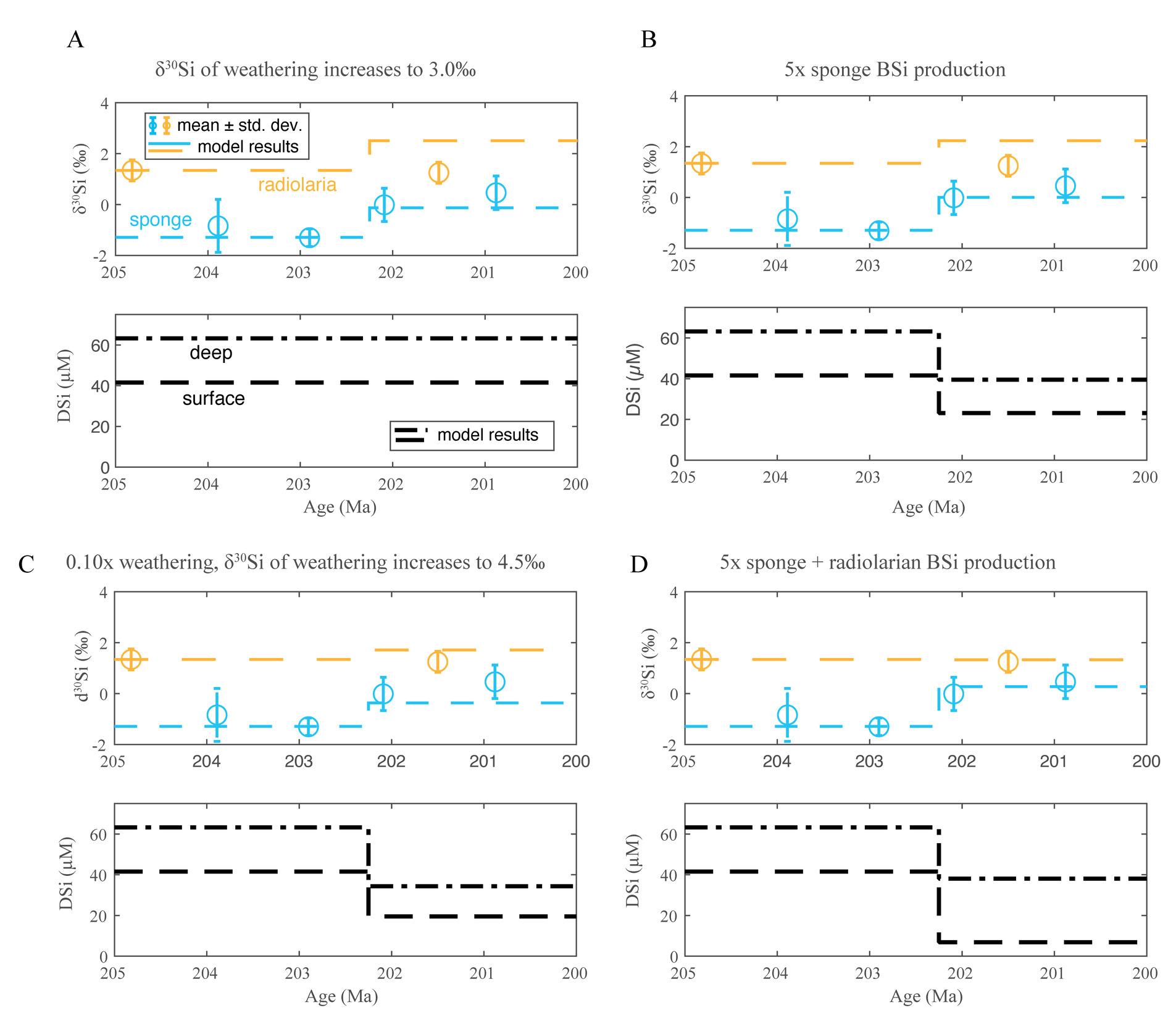
We tested changes to the flux derived from continental weathering (implemented by changing the F_riv term), the isotopic composition of this riverine flux, and sponge and radiolarian BSi production (by changing $V_{max,30Si,sponge}$ and/or $V_{max,30Si,rad}$). These represent the changes most consistent with other geological evidence from the time, including global changes in weathering in the leadup to and associated with the Triassic–Jurassic Boundary (Heszler et al., 2024; Kuroda et al., 2010), changes in stable carbon isotopes of organic matter (Yager et al., 2017), and changes in sponge abundance in shelf ecosystems (Ritterbush et al., 2014, 2015). We identified the changes to these parameters that could explain the observed shift in δ³⁰Si of sponge spicules, and we evaluated the associated effect on radiolarian δ³⁰Si (fig. 10).

Several scenarios can explain the change in sponge spicule δ³⁰Si, but several also produce a change in radiolarian δ³⁰Si that do not obviously match the limited observations available. For example, an increase in the δ³⁰Si of weathering inputs from 1.25‰ (the starting condition) to 3.0‰ in the model leads to an increase in sponge spicule δ³⁰Si similar to that observed, but with a substantial increase in radiolarian δ³⁰Si. Such increases do not seem compatible with the available radiolarian δ³⁰Si data. Adding a large decrease in weathering flux (to 10% of the starting value) reduces the change in radiolarian δ³⁰Si, but such large changes in the weathering flux are unlikely, and this scenario produces model results that are only just consistent with the data.

An increase in BSi production by sponges alone can also explain the change in sponge spicule δ³⁰Si, but again requires a coincident change in radiolarian δ³⁰Si. In this case, the modeled change in radiolarian δ³⁰Si falls just outside the expected uncertainty on the available data (~0.8–1‰), but given the limited extent of available data, it would be premature to rule out this scenario altogether. Although we cannot exclude other possibilities, the model perturbation that appears most compatible with the data is an increase in BSi production by both sponges and radiolarians, leading to DSi drawdown and increase in sponge spicule δ³⁰Si. Such increased productivity can explain the record on its own (fig. 10), or in tandem with changes in the weathering flux, which are also consistent with the ⁸⁷Sr/⁸⁶Sr records from the same time interval (fig. 11; Heszler et al., 2024; Kovács et al., 2020).

We tested the effect of starting from other steady state configurations that also fit the end-Triassic data (i.e., initial parameters other than those in Supplementary Table 3) and found that details of the required perturbation varied, so we caution against quantitative interpretation from our model results. However, even considering other initial configurations, the overall picture remains the same: observed changes in sponge δ³⁰Si across the TJB are most consistent with significant changes in BSi production.

4.5. Implications for environmental changes associated with the end-Triassic extinction

Coincident with δ³⁰Si_sponge changes, the stable carbon isotope record of organic matter (δ¹³C_org) at Levanto undergoes a positive excursion during the TJB interval (fig. 11) consistent with an increase in biological productivity (e.g., Kump & Arthur, 1999; Larina et al., 2021). This change also coincides with a reversal in global marine ⁸⁷Sr/⁸⁶Sr (Heszler et al., 2024; Kovács et al., 2020), suggesting changes in weathering may have contributed to increased productivity via enhanced nutrient delivery to the oceans. These changes precede the earliest dated CAMP basalts, pointing to significant biogeochemical perturbation in advance of the ETE and CAMP emplacement. The connections between weathering intensity, CAMP activity, biological productivity, and the ETE warrant future investigation, but our results are consistent with conditions favoring high BSi production prior to the end-Triassic and the eruption of the main stages of CAMP. These conditions may have created an opportunity for siliceous sponge proliferation when corals disappeared from shelf habitats (Ritterbush et al., 2014, 2015). Further work investigating other periods of widespread sponge reefs (and other major changes in Si users in the ocean) may also aid in our understanding of sponges’ role in the Si cycle. Multiple “glass ramp” episodes are documented in the Phanerozoic geological record (Ritterbush, 2019), and these could be ripe for further exploration using the sponge Si isotope proxy. Ritterbush (2019) and Alvarez et al. (2017) found that sponge distribution is correlated with both DSi and depth (which are closely related in the modern ocean), and both studies emphasized that DSi alone may not lead to increased sponge proliferation. Instead, other factors such as the decimation of carbonate producing ecosystems in shallow water at the TJB may have resulted in niche opening for sponges and subsequent proliferation. While our study focuses on the Triassic–Jurassic boundary, the evidence for low DSi during the mid-Mesozoic suggests much more work is needed to understand the coupled C and Si cycles and their interplay with ecological communities and biogeochemical cycling. In addition, incorporating more siliceous organisms into Earth system models such as cGEnIE will help to probe aspects of depth dependency, ocean circulation, and biosilicifier impact on DSi and could complement further data collection (e.g., Naidoo-Bagwell et al., 2024).

5. CONCLUSIONS

We measured the δ³⁰Si of 130 sponge spicules from across the Triassic–Jurassic boundary at two stratigraphic sections in Peru to constrain dissolved marine silica concentrations during this time interval. Results reveal isotopic compositions of sponge spicules strikingly similar to the modern, implying DSi was not markedly higher in the mid-Mesozoic unless seawater δ³⁰Si was dramatically different. Radiolarian δ³⁰Si from this time interval, based on prior work in Japan, suggests that was not the case. We therefore conclude that mid-Mesozoic DSi was broadly similar to the modern, adding to growing evidence of significant surface ocean drawdown of DSi even prior to expansion of diatoms. We used a box model to evaluate the silica cycle dynamics required to explain the observed δ³⁰Si data. Baseline results (205–202.25 Ma in fig. 11) confirm that the isotopic signature and mass balance of DSi in the oceans is consistent with the observed δ³⁰Si_sponge and δ³⁰Si_radiolarian data when considering physically and biologically plausible parameters.

In our data, sponge spicule δ³⁰Si values shift from about –1.0‰ in the Late Triassic to about +0.5‰ in the Early Jurassic while radiolarian δ³⁰Si values from Japan remained relatively stable (fig. 11). These changes are best explained in our model by imposing an increase in surface ocean biogenic silica (BSi) production by a combination of radiolarians and sponges, which drive drawdown of DSi from the surface ocean. We cannot rule out BSi production by sponges alone, although such a change would drive a larger increase in radiolarian δ³⁰Si. Model scenarios invoking changes in the magnitude or isotopic composition of the weathering flux to the oceans do not obviously reproduce the data, but some change in weathering flux, as might be expected to drive increased productivity, is compatible with the data if accompanied by increases in BSi production. Overall, our results are consistent with the proliferation of sponges across continental shelves around the world across the Triassic–Jurassic boundary (Ritterbush et al., 2014).

Silicon isotope ratios from sponge spicules spanning the Triassic–Jurassic boundary thus point to a mid-Mesozoic ocean with low seawater DSi resulting from radiolarian and sponge proliferation and subsequent water column drawdown, and a system sensitive to perturbation in ways that may have profoundly affected marine ecosystems during major CO₂ injection and global warming. We caveat these interpretations on the basis that more work is needed to confirm the diagenetic effects on sponge spicule silicon isotope composition, and we also encourage additional effort to build datasets of sponge and radiolarian δ³⁰Si from other locations. Much like Trower et al. (2021), we found it challenging to identify well-preserved spicules and radiolarian tests in the same samples, yet paired records would help to quantify DSi more robustly and to more confidently interpret changes over intervals such as the TJB. The linked C and Si cycles are important to global climate, and better constraining the oceanic DSi content is vital to understanding the coupled evolution of ecological and climatic systems through time. Our results suggest reconsideration of oceanic DSi during the Mesozoic is warranted to accurately represent the global C and Si cycles during deep time.

ACKNOWLEDGMENTS

We thank Yunbin Guan for SIMS instrument tuning and setup and helpful discussions, Kathy Omura at the Los Angeles Natural History Museum for modern sponge samples, and Kate Hendry for providing the modern data compilation in figure 8 and helpful advice. We acknowledge support from the NSF Earth Life Transitions program (1338329), the Caltech Center for Evolutionary Sciences (to WWF), and from the Elizabeth and Jerol Sonosky Fellowship of USC (to JAY). We thank Jessica Whiteside, Terry Isson, and seven anonymous reviewers for their helpful comments on earlier versions of this manuscript.

AUTHOR CONTRIBUTIONS

J.A.Y., K.R., A.J.W., W.W.F., F.A.C., D.J.B., W.M.B., and S.R., designed the study; J.A.Y., E.J.T., and A.J.C. performed the analyses; J.A.Y., A.J.W., E. J. T., and W.W.F. analyzed the data; A.J.W. performed the modeling; and J.A.Y. and A.J.W. wrote the paper, with contributions from all co-authors.

SUPPLEMENTARY INFORMATION

https://doi.org/10.5061/dryad.dfn2z35bq

Editor: C. Page Chamberlain, Associate Editor: Kimberly Lau