1. Introduction
Understanding how faults behave on a range of timescales is crucial for interpreting and mitigating seismic hazards. The Wasatch Fault in Utah, USA, is particularly important in this regard, as a seismically active, surface rupturing, multi-segment fault that strikes along many of Utah’s largest cities. As such, extensive research on the Wasatch Fault has been aimed at quantifying slip rates on short timescales to aid interpretation of seismic hazards (Chang et al., 2006; DuRoss et al., 2018; Valentini et al., 2020; Verdecchia et al., 2019). At the same time, the Wasatch Fault marks the western boundary of the Wasatch Range, a prominent mountain range bounding the Basin and Range province in the east. Hence, over the timescales of 10s of millions of years, the range is interesting from the perspective of understanding how extension in the Basin and Range initiated, developed and continues to occur. For this reason the long-term rock uplift rate history of the range has also been well quantified (P. A. Armstrong et al., 2003; Ehlers et al., 2003; Friedrich et al., 2003).
River networks respond to changes in climate and tectonics, ensuring the Earth’s surface remains in a quasi-equilibrium state. To achieve this, rivers can change aspects of features, such as steepness or width (Goren et al., 2014; Whittaker et al., 2007) or increase their upstream drainage area through capture (Willett et al., 2014), which can drive either erosional or aggradational responses. The consequence of this behavior is that river attributes encode information about spatial and temporal variability in the processes that shape the Earth’s surface (Demoulin et al., 2017; Whittaker, 2012). Typically, river networks encode rock uplift rate information on the 104 to 107 year timescale (e.g., Fox, Bodin, et al., 2015; Goren et al., 2014; Racano et al., 2021; Roberts & White, 2010; Wang et al., 2022), allowing inference of a variety of tectonic processes from faulting in the upper crust (Goren et al., 2014; Lavé & Avouac, 2000; Whittaker et al., 2007) to mantle dynamics (Roberts et al., 2018). Provided we can effectively deconvolve these signals, river network inversions can provide an ideal intermediary between the presently well documented short- and long-term rock uplift rate histories on the Wasatch Fault.
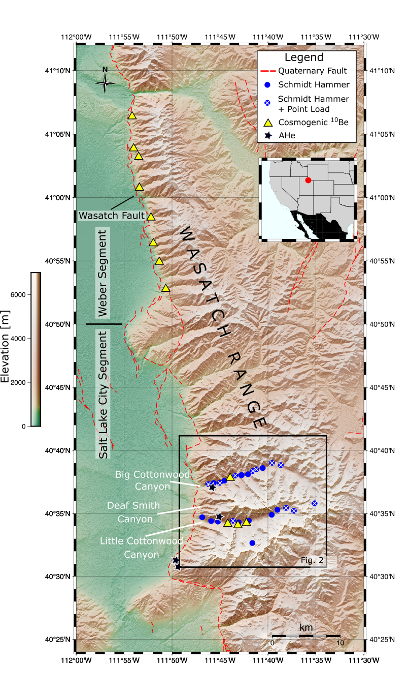
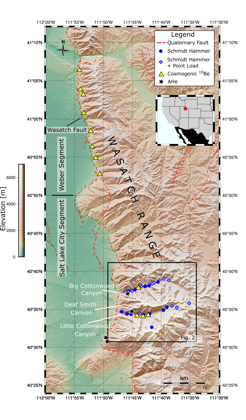
In this study, we investigate three river networks that cross the Salt Lake City segment of the Wasatch Fault (fig. 1). The three catchments are of different sizes, have different glacial histories (Quirk et al., 2020), and incise different bedrock lithologies (Bryant, 2003). This is useful, as commonalities between river networks are likely to be caused by the geological feature they all share: the Wasatch Fault. Having examined the geology and geomorphology of the catchments, we use river network inversions to correlate sections of high and low slope with respect to time, providing a 1 Ma rock uplift rate history of the Wasatch range. We employ a number of new field observations as well as previously published data sets to constrain the stream power model parameters and justify our model assumptions. We are able to reconcile estimates of the erodibility from multiple methods and data sets, which, given that values for the same regions can often vary by orders of magnitude (e.g. McNab et al., 2018; Racano et al., 2021), provides confidence in our inverse model. We find that the rock uplift rate on the Wasatch Fault has varied over the past million years, approximately in tempo with pluvial lake development on the fault hanging wall. Our study supports the theory that unloading and loading cycles of pluvial lakes on the hanging wall could be responsible for accelerations in rock uplift rate on the Wasatch fault (Hampel & Hetzel, 2006; Hetzel & Hampel, 2005).
1.1. Regional Geology
The Wasatch Fault represents the dividing line between the Basin and Range, an active extensional province, and the relatively stable Colorado Plateau. The fault inherits its structure from the Sevier Orogenic Belt (R. L. Armstrong, 1972), which was inverted when extension of the Basin and Range initiated in the Miocene (Cassel et al., 2014; Colgan & Henry, 2009; McQuarrie & Wernicke, 2005). The Wasatch Fault also forms the western boundary of the Wasatch Range, a N-S trending, 400 km long range with elevations exceeding 3500 m (fig. 1). Due to its location on the margin of an asymmetric rift, the Wasatch Fault has accommodated large amounts of strain during the development of the Basin and Range, and hosts some of the highest contemporary strain rates in the region (Chang et al., 2006; Hammond et al., 2014; Long, 2019; Richter et al., 2021).
Normal sense displacement along the Wasatch Fault has likely occurred at least since 17 Ma (P. A. Armstrong et al., 2003, 2004; Ehlers et al., 2003), however measured displacement rates during this time have been variable with different studies producing different and sometimes contradictory results (P. A. Armstrong et al., 2003; Ehlers et al., 2003; Jewell & Bruhn, 2013; Karow & Hampel, 2010; Machette et al., 1991; Mayo et al., 2009). Increases in slip rate along the Wasatch Fault during the Holocene have been suggested based on numerical modeling (Hetzel & Hampel, 2005; Karow & Hampel, 2010; Mattson & Bruhn, 2001), and field studies using paleoseismic data (DuRoss et al., 2018; Mayo et al., 2009). Over longer timescales, rock uplift of the Wasatch is reported to have decreased, with thermochronology data and modeling suggesting rock uplift rates have changed from 1.2 mm year−1 between 10 and 5 Ma to 0.8 mm year−1 from 5 Ma to recent times (Ehlers et al., 2003; Stock et al., 2009). Reconciling the recent and long-term data is thus difficult, owing to the disparate timescales over which rock uplift rates are recorded, and the multitude of processes that can be responsible for changing rock uplift rates along the Wasatch. For instance, longer term variation is suggested to be caused by changes in large tectonic structures, such as the movement of the structural hinge of the fault, or fault segmentation and linkage (P. A. Armstrong et al., 2003; Ehlers et al., 2003) whereas short term variation has been attributed to a number of mechanisms, including flexure from glacial loading and changes associated with earthquake clustering and seismicity cycles (Biemiller & Lavier, 2017; Hampel & Hetzel, 2006; Hetzel & Hampel, 2005; Machette et al., 1991; Malservisi et al., 2003; McCalpin & Nishenko, 1996; Pérouse & Wernicke, 2017).
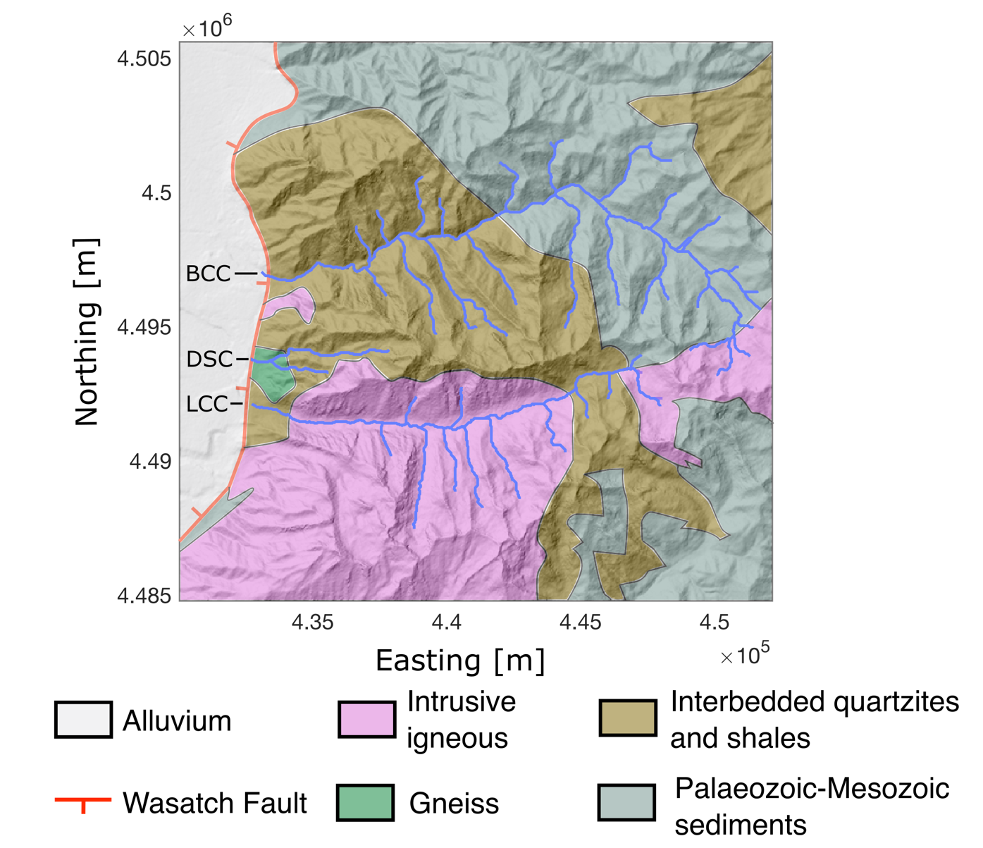
This study focuses on the Salt Lake City segment of the Wasatch Fault, which is situated in the middle of the Wasatch Fault zone (fig. 1). The southern portion of this segment has significantly younger apatite (U-Th)/He ages than the rest of the range, equating to exhumation rates more than twice as fast as the northern part of the segment, and adjacent segments (P. A. Armstrong et al., 2004). We study the three river networks that cross this section of the fault; Big Cottonwood Canyon, Little Cottonwood Canyon, and Deaf Smith Canyon. The networks are adjacent to each other, yet all incise different lithologies (fig. 2). The intrusive igneous rocks of the Little Cottonwood stock dominate the bedrock lithology of Little Cottonwood Canyon. However, they are almost entirely absent from Big Cottonwood Canyon, which incises a series of limestones and marbles in the upstream portion, and quartizites and interbedded shales and siltstones downstream. Deaf Smith Canyon, being between the two larger catchments, incises the intrusive igneous rocks in its southern tributaries, the interbedded quartzites in the trunk stream, and Precambrian Gneiss downstream close to the Wasatch Fault.

The three catchments also differ in their glacial histories. Modeling of past glaciation from the extent of mapped morraines shows that Little Cottonwood Canyon was the most extensively glaciated of the three catchments at the peak of the last glacial maximum (LGM, 26 – 19 ka), with glaciers terminating at the Wasatch Fault (Quirk et al., 2018, 2020). Big Cottonwood Canyon glaciers were less extensive, and approximately 100m thinner than the Little Cottonwood Canyon glaciers at comparable locations along the trunk streams (Quirk et al., 2018). As a result, glaciers in Big Cottonwood Canyon did not extend to the downstream portion of the fluvial network. Furthermore, during the Lateglacial (19–12 ka), although ice was present in Little Cottonwood Canyon, it was almost entirely absent from Big Cottonwood Canyon. The smaller Deaf Smith Canyon hosted less than 100 m of ice during the LGM, which receded during the Lateglacial similar to Big Cottonwood Canyon (Quirk et al., 2020).
_and_little_cottonwood_canyon_(lcc)__with_cross_secti.png)
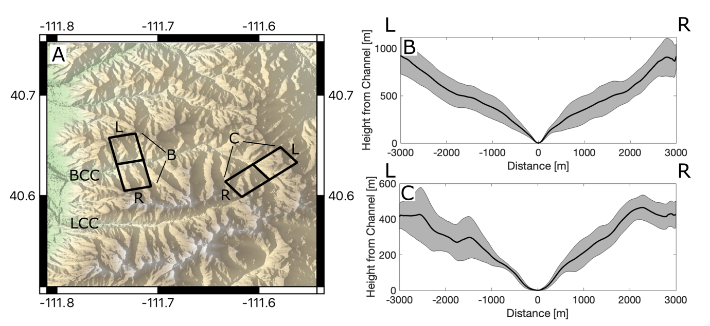
During the LGM, the equilibrium-line altitude (ELA) of Little Cottonwood Canyon was approximately 2500 m (Laabs et al., 2006), and in adjacent catchments the ELA would likely be similar. Whilst glaciers can be effective agents of erosion above and at the ELA, below the ELA glaciers have little incisional power (Brocklehurst & Whipple, 2006; Fox, Leith, et al., 2015; Leith et al., 2014; Petit et al., 2017). Although it is possible that the ELA was lower in our catchments during previous glaciations, there is evidence that glaciation has not significantly changed the hypsometry of the catchments below approximately 2400m. Above approximately 2400 m, the catchments do present U-shaped, glacially eroded valleys (fig. 3C), however, downstream of 2400 m, the valleys look fluvially incised, with a distinctive V shape (fig. 3B). To minimize the influence of glaciation on our study, we focus on the fluvial, downstream portions of each catchment, below approximately 2400 m.
2. Methodology
We extract signals of rock uplift rate from river networks crossing the Wasatch Fault. However, a host of processes such as lithology, climate and faulting can influence the shape of a river network. In order to have confidence that the signals we infer are indeed related to rock uplift, we must also examine the signals that we expect to be present due to these processes. We investigate spatial differences in relative rock uplift rate using the steady state stream power model, and quantify differences in bedrock lithology by measuring the uniaxial compressive strength of bedrock samples using Schmidt hammer and point load test measurements. We also investigate how erodibility has changed in both space and time using previously published cosmogenic 10Be data and a method to recover erodibility from river networks directly.
2.1. The Stream Power Incision Model
Rock uplift and erosion are the two fundamental processes responsible for changing the elevation of the Earth’s continents. For any given point, the change in elevation with respect to time, can thus be expressed as a balance between the rock uplift rate, u, and erosion rate, E, that the point has experienced. This can be written into the following simple equation,
∂z(x,t)∂t=u(x,t)−E(x,t),
where x represents the spatial coordinate of a point, and t represents time.
For a point on a river network, the erosion rate can be determined using the stream power incision model (SPIM), (Howard & Kerby, 1983; Whipple & Tucker, 1999), which states that,
E=KAmSn
where E is bedrock channel erosion, K is the erodibility which accounts for factors such as climate and geology, A is the upstream drainage area, a proxy for discharge, and S is the slope of the channel. Upstream drainage area and slope are raised to the powers of m and n respectively, for which a range of appropriate values have been suggested based on theoretical predictions (Whipple & Tucker, 1999), empirical observations (Snyder et al., 2000), and numerical modeling (Gasparini & Brandon, 2011). Equation (2) can then be substituted into equation (1), to give the following expression, describing elevation change at a point on a river network with respect to space and time,
∂z(t,x)∂t=u(t,x)−KA(x)m(∂z(t,x)∂x)n,
where the slope, S, is denoted and upstream drainage area, A, is temporally invariant.
If we make the assumption that a catchment is in steady state, i.e., that rock uplift and erosion are equal, we can extract the relative rock uplift rate, or channel steepness index (ks), by rearranging equation (3) to
ks=(uK)1n=A(x)mn(∂z(t,x)∂x),
where m/n is the concavity index, or θ. is the channel steepness index, ks, which provides a quantitative measure of rock uplift from measurable river properties.
2.2. The Integral Approach to Calculating Spatially Variable Channel Steepness Index
Although first noted by Hack (1957) and Morisawa (1962) the slope-area relationship described by equation (4) was formalized by Flint (1974), which states that,
dzdx=ksA−θ.
Whilst it is possible to infer channel steepness index with slope and upstream drainage area, when working with noisy topographic data, using the derivative of elevation, slope, accentuates this noise and so is disadvantageous. To work directly with the elevations, we can integrate equation (5), so that
z(x)=zb+ks(x)Aθ0χ(x),
where χ is an integrand, defined as,
χ=∫xxb(AoA(x))θdx.
Here, z is the steady-state elevation of a point, x, zb is the baselevel elevation, and A0 is a reference drainage area. Equation 6 describes provides the basis of the integral approach (Harkins et al., 2007; Perron & Royden, 2013; Royden et al., 2000) under a steady-state assumption, and the assumption that both rock uplift and erodibility are spatially invariant.
The method we apply to the river networks of the Wasatch is described by Fox (2019) and Smith et al. (2022), and can infer spatially varying channel steepness index, and thus rock uplift and erodibility. This is achieved by discretizing the river network into nodes separated by small blocks of χ, where the value of channel steepness index within each block is forced to be the same, but values of channel steepness index can vary from block to block. As we are inferring channel steepness index parameters, the methodology is totally independent of any assumptions about the erodibility, K, or the slope exponent n (eq 4). Prior to analysis, river network elevations are normalized to baselevel, taken as the point where each network crosses the Wasatch Fault, and A0 is set to 1 m2. We can then describe the elevation of a given river network node, k, as a summation of the small blocks of χ and the ks value within each block, such that,
[ΔχiΔχjΔχk][kiskjskks]=zk,
where i, j, and k represent consecutive river network nodes from the baselevel to node, k, and ks and ∆χ represent the channel steepness index between each node and the blocks of χ respectively. In this example, the sum of ∆χ values is equivalent to the χ value at node k. Writing this summation for each node in the network and combining them into a matrix of size n × n where n is the number of river nodes in the network, we can infer channel steepness index values by taking the inverse of this matrix and a column vector of river node elevations. Smoothness constraints can also be incorporated into this system, ensuring that channel steepness varies realistically in space (Fox, 2019; Smith et al., 2022). In this study, we use a Laplacian operator similar to the one described in section 2.4.
To calculate χ, and thus channel steepness, we must estimate a value for the concavity index, θ. Although empirical studies to constrain the concavity index are often contaminated by spatial gradients in either rock uplift or climate, studies in catchments where these effects can be controlled find that values fall between a narrow range of 0.4 and 0.6 (Kirby & Whipple, 2012). Previous studies have leveraged the χ transformation to more tightly constrain θ, by acknowledging that if an area is in steady state, the trunk stream and tributaries of a river network should be colinear on a χ-plot (Goren et al., 2014; Mudd et al., 2014; Perron & Royden, 2013). In the Wasatch however, interpretation of thermochronometric data suggests a pattern of decreasing rock uplift rate away from the fault (P. A. Armstrong et al., 2003), which can be due to either tilt of the fault around a structural hinge, or flexure. Therefore, the trunk streams of the river networks draining the range perpendicular to the fault should have χ profiles that decrease in gradient upstream. Alternatively, the tributaries, which are broadly parallel to the fault will experience the same uplift rate along their course, and thus have straight χ-profiles tangential to the trunk stream. As a result, it would be inappropriate to estimate the concavity index by collapsing the χ-profile. Instead, we have assumed a value of 0.45 throughout our analysis, resulting in the calculation of the normalized channel steepness index, ksn (Smith et al., 2022). This value is consistent with values used in studies in similar tectonic settings (see Gailleton et al., 2021; Kirby & Whipple, 2012; Smith et al., 2022 for further discussion), but we do investigate how the choice of concavity index influences our results, and why it would be unlikely to change our interpretations (supplementary material 3).
2.3. Recovering rock uplift rates from stream networks using the K-independent analytical solution to the stream power model
Equations 1–8 show that, under steady state conditions, the elevation at each point on a river network is a function of the relative rock uplift rate that point experiences. Channel steepness index can be extracted using the integral approach and can be a useful tool for investigating spatial variations in relative rock uplift rate. However, river network elevations are also a function of rock uplift rate with respect to time, and so channel steepness index not only represents spatial variation in relative rock uplift rate, but temporal variation in rock uplift rate. In the Wasatch, the river networks that cross the fault are relatively small, whilst the long term rock uplift rates are relatively high (P. A. Armstrong et al., 2003; Ehlers et al., 2003), therefore, we may expect temporal variation in rock uplift rate on the Wasatch Fault to dominate local variation in channel steepness index. It is thus useful to infer the rock uplift rate history recorded by the rivers that cut the Wasatch Fault. To do this, we use the methodology outlined in Goren et al. (2014), which is based on the transient linear stream power incision model (eq 3). One key assumption we make is that the value of the slope exponent, n, is 1. The validity of this assumption is tested in section 4.3.
Although possible in some unique landscapes (Ferrier et al., 2013), the determination of the erodibility, K, is difficult. To allow us to extract rock uplift rates without constraining K, we assume that K is invariant through time, and constant throughout any given river network. We allow K to vary between networks, and the importance of this is discussed in section 4.2. Given this assumption, we can then make the following variable transformations,
t∗=tKAm0,
and
U∗=uKAm0,
where t* has the units of length, and U* is dimensionless. Introducing these transformations into equation (3), we can write,
∂z(t∗,x)∂t∗+(A(x)A0)m∂z(t∗,x)∂x=U∗.
The solution to equation (11), developed in (Goren et al., 2014), therefore takes the form,
z(t∗,x)=∫t∗t∗−χ(x)U∗[t′,τ−1∗(χ(x)−t∗+t′)]dt′,
where represents the response time, or the time taken for the channel to respond to changes to rock uplift rate. This is related to χ by the following equation,
τ(x)KAm0=χ(x).
To infer the dimensionless rock uplift history experienced by the river networks of the Wasatch, we follow the inverse scheme defined by Goren et al. (2014) that also accounts for spatial variability in the rock uplift rate on the fault due to flexure. This system of equations takes the form,
A∗sBλU∗=z,
where z is a column vector of river network elevations for each river node, so that the number of rows is equivalent to the total number of nodes, N , defined in the river network. U∗ is a column vector that defines the dimensionless rock uplift rate history, so that each row in U∗ is the U* value at a given timestep, where the total number of timesteps q, is defined by the discretization of χ.
is the model matrix, of dimensions N × N · q. Each row in the A-matrix corresponds to a node in the river, and each column has the value of either ∆χ or 0. The row is filled such that, at each timestep, the sum of ∆χ values is equal to the χ value of the node. An algorithm to fill the A-matrix is given in Appendix C of Goren et al. (2014).
The matrix parameterizes the spatial variability in rock uplift rate away from a fault. We expect rock uplift to decay away from the surface trace of the fault due to flexure, according to the following equation,
((fU∗i=(fU∗0exp(−diλ)cos(diλ),
where f represents the timestep, and i represents the river node. is the dimensionless uplift rate at the fault, and di is the distance between the fault and the river node, i. is a flexural parameter, given by the following equation,
λ=(ETe33(ρm−ρc)g(1−ν2))0.25,
where E is the Young’s modulus, in this study set to 70 GPa, Te is the effective elastic thickness, set to 16 km, based on values from previous studies (Austermann et al., 2020; Lowry & Smith, 1994; Malservisi et al., 2003), ν is Poisson’s ratio, set to 0.25, and and are the densities of the mantle (3300 kgm−3) and continental crust (2900 kgm−3) respectively. g is gravity, set to 9.81 ms−2.
is an matrix, where each row contains one non-zero entry. In the first column, representing the first timestep, the rows 1 to N contain the non-zero entries evaluated from,
exp(−diλ)cos(diλ).
In the second column, which represents the second timestep, the same non-zero entries for each river node are input in rows N +1 to 2N, and so on. In this way, at each timestep, variation in the relative rock uplift rate due to the distance of each river node from the fault is accounted for.
Multiplying and produces a matrix, of dimensions where each row represents a spatially parameterized river node. This allows us to recover the dimensionless rock uplift rate at each timestep, q, to recover the rock uplift rate history. Under certain conditions, this can be calculated as,
A∗λ−1z=U∗.
2.4. Implementing smoothing constraints
The model described by equation (18) is mixed determined, as the number of river network nodes constraining each timestep in the rock uplift rate history model varies. More recent timesteps are generally characterized by a greater number of river network nodes, and so are overdetermined. However, there are fewer points on the network that survive and represent long response times, and so early timesteps in the rock uplift rate history can be underdetermined (Menke, 2012). To solve a mixed-determined problem, we use a least squares method with a form of regularization. The regularization we use is a Laplacian operator, which controls the smoothness of the rock uplift rate parameters (Constable et al., 1987), The smoothness around a timestep is described as,
∇2U∗p= 2×U∗p−U∗p−1−U∗p+1,
where is the U* value at timestep p. Incorporating equation (19) into the model described in equation (18), the system takes the form,
(A∗λ…α∇2)U∗= (z…0),
Where α is a scalar, that can be used to increase or decrease the importance of smooth model parameters to the solution. At greater values of α, smoothness is prioritized, whereas at lower values, the model fit to the data is prioritized. To inform an appropriate choice of α, we perform a resampling test and investigate the model misfit across a range of values of α (see section 3.2).
2.5. Model Calibration and Estimating Erodibility
The model described in equation (20) allows inference of a dimensionless rock uplift rate history, or U* from river networks. However, we can derive the rock uplift rate history from U* and t∗ by transforming them according to equations (9) and (10). To estimate a value of K, we find the value of K that causes the exhumation predicted by the inferred rock uplift rate history of Little Cottonwood Canyon to match the rock uplift rate predicted by thermochronometric data from the same catchment (P. A. Armstrong et al., 2003; Ehlers et al., 2003) over a million year time period. We use the thermochronometric data rather than the erosion rate data derived from cosmogenic nuclides (Stock et al., 2009) for two reasons. Firstly, the thermochronometric data covers the entire Little Cottonwood Catchment, whereas the erosion rate data only sample 3 smaller catchments within Little and Big Cottonwood Canyon. Secondly, the river networks record incision on the km scale, similar to the amount of exhumation recorded by the thermochronology, whereas the cosmogenic 10Be-derived erosion rates only record a few meters of denudation. It is therefore more appropriate to calibrate our networks with the constraint that records exhumation on a similar scale to that recorded in our networks.
Importantly, we allow the K values used to calibrate the normalized rock uplift rates to vary between networks. To do this, we minimize the misfit between the dimensionless rock uplift rate histories from catchments for which there is not thermochronometric data, and the calibrated rock uplift rate history from Little Cottonwood Canyon, by adjusting K based on a ratio to the K value used for Little Cottonwood Canyon. Note that we expect K to vary spatially due to the different bedrock lithologies of each catchment. The inferred contrast in bedrock hardness and erodibility in each catchment can be validated using field measurements of rock strength and previously published cosmogenic 10Be denudation rate data, described below.
2.5.1. Schmidt Hammer Measurements
Variations in bedrock strength and climate may have profound impacts on the erodibility of a catchment, influencing sediment supply, resistance of bedrock to abrasion or ability of bedload to erode (Baynes et al., 2020; Bernard et al., 2021; Sklar & Dietrich, 2001, 2006). In our study area, the climates of each catchment are similar, but the bedrock lithologies are different. Quantifying bedrock strength is thus important to our study to understand how erodibility may vary within each catchment as a result of lithology. To do this, we use the Schmidt hammer, a portable field instrument that can be used to obtain a large number of measurements of bedrock strength across our catchments of interest (Bolla & Paronuzzi, 2021; Saptono et al., 2013). Measurements were made on bedrock outcrops at regular (approx. <1 km) intervals adjacent to the trunk streams in Big and Little Cottonwood Canyons, where exposure allowed (fig. 1). At each locality, greater than 20 Schmidt hammer measurements were obtained, and the lowest 50 % of measurements discarded, in accordance with International Society for Rock Mechanics (IRSM) guidelines (Aydin, 2008). To convert the Schmidt hammer rebound numbers into rock strength (here quantified as the Uniaxial Compressive Strength, UCS), we use equation (21), following Deere and Miller (1966) and Saptono et al. (2013), where,
UCS=6.9 × 100.00087ρR+0.16.
Here, ρ is rock density in g cm−3 and R is the rebound value. We note that while rock abrasion rates experimentally scale with tensile strength (Sklar & Dietrich, 2001, 2004), other factors such as sediment supply (Sklar & Dietrich, 2004; Turowski et al., 2007), grain size, joint spacing (Chilton & Spotila, 2022) and the ratio between bedload and bedrock strength (Fox et al., 2023) influence erosion rates. Furthermore, uniaxial compressive strength and tensile strength are related to one another in Mohr-Coulomb space, thus we elect to describe rock strength using the more commonly reported uniaxial compressive strength metric.
2.5.2. Point Load Tests
Several empirical equations exist to convert the Schmidt hammer rebound value, R, into uniaxial compressive strength (Saptono et al., 2013), illustrating the uncertainty in predicting UCS from the Schmidt hammer measurements. Therefore, to increase confidence in our estimates of rock strength, we performed point load tests on irregular hand specimens obtained from field outcrops, which tend to more accurately predict UCS (Singh et al., 2012).
At 11 of the 26 Schmidt hammer locations, five to ten approximately 15 × 8 × 5 cm sized rock samples were collected for point load testing at the University of Utah. Point load tests were performed following ISRM guidelines (Franklin, 1985), and the two highest and two lowest results were discarded for each lithology. In total, there were 15 UCS data points generated for the granodiorite of Little Cottonwood Canyon and 11 values generated for the quartzites of Big Cottonwood Canyon.
2.5.3 Channel Steepness Index – Erosion Rate Relationships
Although bedrock strength is likely to influence erodibility, the mechanisms that cause lithology to affect erodibility are generally poorly understood. Fortunately, we can use a previously published 10Be cosmogenic nuclide data set to further infer spatial variation in erodibility. This can be done by substituting Flint’s law (eq 5) into the detachment limited SPIM (eq 2), to produce the following relationship between the normalized channel steepness index and erosion rate,
E=K⋅ksn.
Here, normalized channel steepness index, ksn, refers to channel steepness index that has been measured using the same reference m/n or concavity index value. From this equation, we can see that a plot of channel steepness index vs erosion rate should provide a relationship where erodibility, K, can be constrained from the gradient.
We calculate the basin wide average normalized channel steepness index value for 11 catchments along the Wasatch Fault, using the above described methodology (section 2.2), and compare these to the existing basin wide erosion rate data set inferred from cosmogenic 10Be nuclide data (Stock et al., 2009). We fit a regression, forced through the origin, of these data to provide a constraint on K for different catchments and groups of catchments, which allows us to assess whether erodibility varies spatially. The value of erodibility inferred from this relationship also allows us to assess whether our estimate of erodibility derived from the calibration of the relative rock uplift rate histories inferred from the river networks is reasonable.
2.6. Assessing Temporal Variations in Erodibility
The erodibility values between Big Cottonwood Canyon and Little Cottonwood Canyon are expected to be different due to lithology, and we attempt to quantify how much these values vary spatially using field measurements and cosmogenic 10Be data. However, as well as varying in space, erodibility may also change through time due to the influence of changing climate during glacial-interglacial cycles (Belanger et al., 2022). It is therefore important to quantify these potential variations, to ensure our assumption that K is constant through time is justified. To examine how K may have changed, we use a method based on the analytical solution to the linear stream power model, presented by Goren (2016). In this model, erodibility is inferred from the χ values and the response time (ResTime) of the network, by evaluating,
K(t=ResTime(x))= (dχ(x)dResTime(x)).
If the rock uplift rate is known, it can be used to calculate the ResTime for each point on the network. This can be done by discretizing the rock uplift rate in time, which allows the elevation of points on the river network to be described by,
zi= J∑j=1UjΔtj,
where i is a river network node, and j represents discretized time where ∆t is the discrete time interval. The ResTime is the time interval required to evaluate the elevation, zi and is therefore calculated as,
ResTime= J∑j=1Δtj.
Knowing the ResTime and the χ values of the river network, the erodibility at a time, t, can be calculated by differentiating equation (23) numerically, so that,
K(ResTimei+12)= χi+1−χiResTimei+1−ResTimei.
We use the rock uplift rate history inferred by P.A. Armstrong et al. (2003) and Ehlers et al. (2003) to make the ResTime calculation, and thus explore potential K variability through time.
3. Results
3.1. River networks of the Wasatch
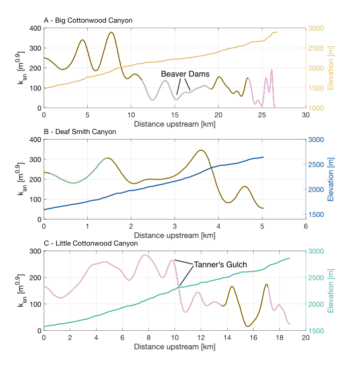
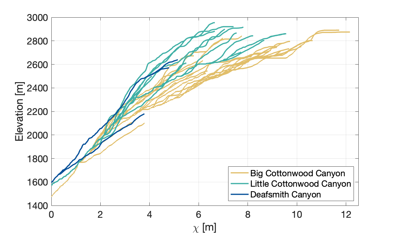
The river profiles of Big Cottonwood Canyon, Little Cottonwood Canyon and the smaller Deaf Smith Canyon are shown in figure 4, along with the channel steepness index as a function of distance along the trunk stream. River networks used in our analysis were extracted from an 30 m SRTM DEM (Farr et al., 2007) using TopoToolbox (Schwanghart & Scherler, 2014). The upstream drainage area required for a point to be considered part of the network is 1 km2, and the baselevel is taken as the point where the rivers cross the Wasatch Fault. The catchments have previously hosted glaciation (Quirk et al., 2020) which has been suggested to limit the ability to infer rock uplift rates from river networks. However, several lines of evidence suggest this is not the case in the Wasatch. Firstly, the present day signature of glaciation can be observed as a flattening of river trunk streams above ∼2500 m elevation, and steep, glacial headwaters, suggesting that only a small portion of the catchment is currently affected by glacial erosion. Secondly, in all three catchments there is a slope break knickpoint that separates a flat, upstream portion and a steeper downstream portion of the river. On a χ-plot (fig. 5), this knickpoint appears at a similar value of χ (approx. 2.5–3 m) in all catchments and is observed not only in the trunk stream but also in the tributaries. This suggests that although past glaciations extended beyond this knickpoint, and even beyond the range front in the case of Little Cottonwood Canyon (Quirk et al., 2020), the vertical component of glacial erosion was not sufficient to remove this feature. This is consistent with observations from previously glaciated fluvial networks in other regions, and with observations of the Big Cottonwood Canyon valley itself (fig. 3; Adams & Ehlers, 2018; Fox, Leith, et al., 2015; Leith et al., 2018; Petit et al., 2017). It is thus more likely that the knickpoint is associated with a temporal change in relative rock uplift rate. Finally, as the glacial histories of each catchment are different, common signals extracted from each river network are unlikely to be associated with glaciation (see section 1.1).


As well as the prominent slope-break knickpoint, there are a series of knickpoints in each of the rivers that create an oscillatory pattern of channel steepness index (fig. 4). These oscillations appear to occur independently of lithology, as they rarely coincide with lithological boundaries (fig. 4). In some cases however, variation can be attributed to geomorphic noise. For example, in the upstream portion of Big Cottonwood Canyon, beavers have created dams flattening sections of the river. These correspond to two sections of low channel steepness index visible in the channel steepness index plot. In the upstream, glacially influenced portions noise can also be created by cyclopean stairs. Even so, the magnitude of this signal is much smaller than the magnitude of changes in channel steepness in the steeper downstream portion of each of the profiles.
In each catchment, two sections of high channel steepness index are preserved in the downstream portion of the network. These zones of high channel steepness are approximately 500–1000 m in length. The nature of these zones of high channel steepness, found across three geomorphically different catchments suggests that they are related to larger scale changes in tectonics or climate. To better understand what may be driving changes in channel steepness index, we use the linear inverse model described in section 2.3 to extract the relative rock uplift rate history of the Wasatch Fault.
3.2. Defining smoothness parameter, α
In order to perform river network inversions, we must define α (eq 20), the inversion parameter that controls the smoothness of the solution. Commonly, this is achieved by plotting an L-curve (Goren et al., 2022), however, due to issues associated with using L-curves (Bodin & Sambridge, 2009), we instead choose to use a form of cross validation (Aster & Thurber, 2013).
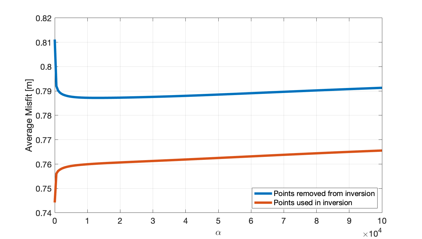
We remove 50 % of the river nodes from the model matrix and infer the dimensionless rock uplift rate parameters. These parameters are then used to predict the elevations of the river network, first for the river nodes included in the model matrix and then for the river nodes excluded from the model matrix. We compare the average misfit between the true elevations of the river nodes and the predicted river node elevations for a range of values of α (fig. 6). For the river nodes included in the model matrix, misfit is expected to increase with increasing α, as fit to the data is sacrificed for solution smoothness. However, for the model parameters derived from the resampled matrix, we expect that at low values of α, the model has little predictive power. There is high misfit between the elevation values of the river nodes removed from the matrix and the predicted elevations of those nodes from model parameters. Gradually as α is increased, misfit is reduced as the predictive power of the model increases, until it reaches a minimum, at which time the misfit increases again as the fit to the data is sacrificed for solution smoothness. The α value that we therefore use, based on figure 6, is 500, which provides the solution with the greatest predictive power and represents a balance between fit to the data and model smoothness.

3.3. Calibration of rock uplift rate history
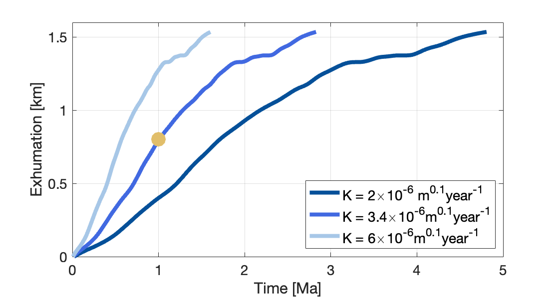
Following the determination of α, the dimensionless rock uplift parameters must be calibrated. This requires finding an appropriate value for K. To do this, we convert the U∗ history inferred from our model into a rock uplift rate history for a range of values for K and iterating so that the exhumation predicted from the rock uplift rate history from the river profiles matches an exhumation constraint predicted by thermochronometry (fig. 7). As the thermochronology samples are from Little Cottonwood Canyon, we match the exhumation predicted from thermochronology to exhumation predicted from the relative rock uplift rate history from the Little Cottonwood Canyon river network (Ehlers et al., 2003).

The total amount of exhumation predicted by the river network is less than the amount of exhumation recorded by an apatite (U-Th/He) sample. We also do not wish to include the exhumation predicted by the upper, glacial portion of the catchment in the calibration. Therefore, we place a constraint at 1 Ma, based on the long-term rock uplift rate of 0.8 mm year−1 derived from thermochronometry (P. A. Armstrong et al., 2003; Ehlers et al., 2003). This spans the timescale of interest and represents the majority of the exhumation recorded by the downstream portion of Little Cottonwood Canyon which we believe represents the most robust estimates of rock uplift (see section 4.1 and 4.3). The K value that matches this exhumation constraint is 3.4 ×10⁻⁶ m0.1year−1 (fig. 7).
3.4. Minimizing misfit between inferred rock uplift rate histories
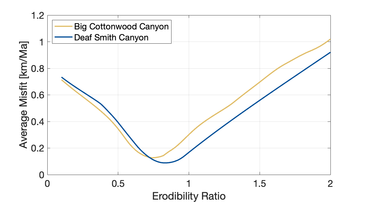
Rock uplift rate histories derived from the three catchments should record the same variation in rock uplift through time. However, given the differences in bedrock lithologies of all three catchments (Bryant, 2003), and the potential differences in precipitation between the Cottonwood Canyons (Campbell & Steenburgh, 2014), it is inappropriate to assume the same K value for all three catchments. We can instead alter the K values between the catchments to minimize the misfit between the derived rock uplift rate histories. We do this by using the predicted K value from Little Cottonwood Canyon, and adjusting the K values of the other catchments based on a ratio. The appropriate K ratio is the value that produces the smallest misfit between the recovered rock uplift rate histories of both catchments (fig. 8). Little Cottonwood Canyon has the highest erodibility value, whereas Big Cottonwood Canyon has an apparent erodibility about 0.75× that of Little Cottonwood Canyon, while Deaf Smith Canyon has an apparent erodibility 0.8× that of Little Cottonwood Canyon. These represent minima of the misfit curves in figure 8.

3.5. Schmidt hammer and point load test data
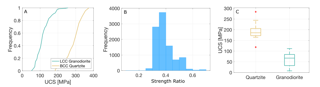
We use Schmidt hammer and point load test data to estimate bedrock strength for the Cottonwood Canyons, which can be used to validate our assumption that the K values of each catchment differ. To simplify the data set, we have included only the dominant rock types in the downstream Big and Little Cottonwood Canyons where the knickzones are located. These are quartzites in Big Cottonwood Canyon, and granodiorite in Little Cottonwood Canyon. We show the Schmidt hammer data for each lithology as cumulative frequency curves in figure 9A. We then calculate the strength ratio between these curves for comparison with the K ratio previously calculated from the misfit. To do this, we select a random frequency value and take the strength value at this point on each curve. We then take the ratio between the quartzite and granodiorite values. This is performed 10,000 times to produce a histogram (fig. 9B). Results from the point load test data are shown as box plots in figure 9C.
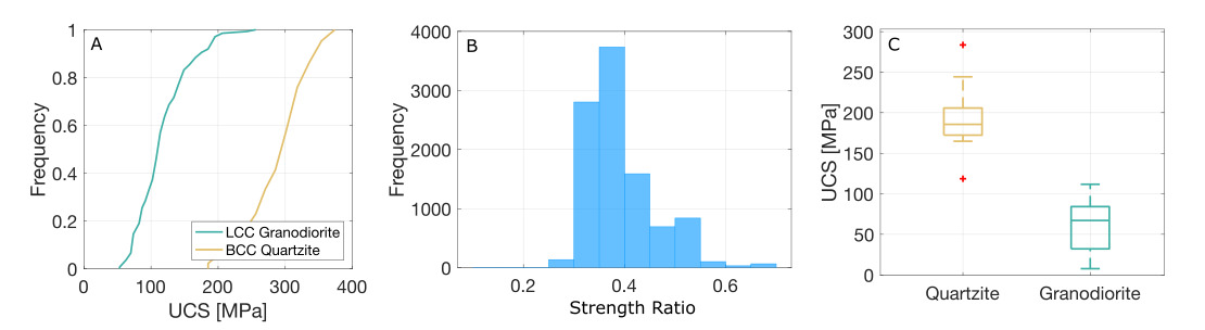
UCS values predicted from both the Schmidt hammer data and point load tests are similar, with the point load data predicting slightly lower UCS values than the Schmidt hammer. Both data sets predict the same trends and show good agreement. There are large differences between the compressive strength of the quartzites and that of the granodiorite (fig. 9). The granodiorites have UCS that is approximately one third that of the quartzites, thus we might expect the erodibility of Little Cottonwood Canyon to be higher than that of Big Cottonwood Canyon. This difference in bedrock strength between the catchments shows that it is necessary to perform the inversion for rock uplift rates separately for each catchment, so we can account for changes in erodibility during the calibration of the normalized rock uplift rate histories (Sections 2.5, 3.4).
The strength ratio predicted from Schmidt hammer data and point load tests is greater than the erodibility ratio predicted by the misfit curves (fig. 8). However, we would not expect these ratios to be the same as erodibility is not controlled solely by bedrock strength. One important factor controlling erodibility is the contrast between bedrock strength and the strength of the impacting particles (Fox et al., 2023; Sklar & Dietrich, 2004). For example, suppose two catchments erode two different lithologies that are homogenous within each catchment. All else being equal, we may not expect the erodibility between each catchment to significantly differ, given that the tools of erosion in each catchment have the same relative efficacy against the bedrock of the river network. Therefore, we can define the following relationship, described by Fox et al. (2023),
K∝KrKs,
where the local erodibility at a point on a river network, K, is related to the contrast between bedload and bedrock strength, Kr is the average bedrock erodibility upstream of the point, and Ks is the bedrock erodibility at the point. In this relationship, Kr is the bedload erodibility, assuming that the bedload represents the average upstream bedrock strength. The term can be multiplied by a scaling parameter to give the actual erodibility values everywhere. In this study, we have used erodibility ratios, hence we remove this parameter to work directly with the bedload/bedrock ratio.
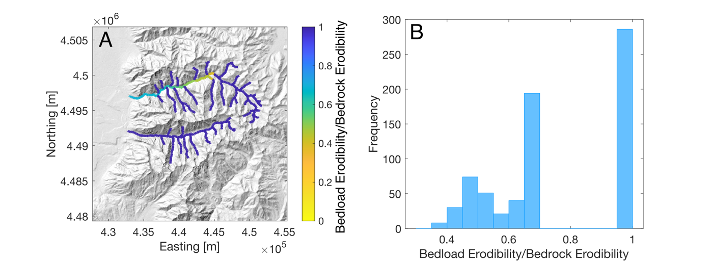
We use the Schmidt hammer measurements to predict the bedload/bedrock erodibility ratio for each point on Big Cottonwood and Little Cottonwood Canyon (fig. 10). We assume a simplified bedrock strength distribution. Little Cottonwood Canyon incises only granodiorite, for which we have UCS estimates from Schmidt hammer and point load measurements. Big Cottonwood Canyon on the other hand incises a mixture of granodiorite and sedimentary rocks upstream, which we assume have the strength of granodiorite, and quartzites in the downstream fluvial portion for which we have UCS estimates. In Little Cottonwood Canyon the bedload/bedrock ratio is 1 everywhere as there is only one rock type in the catchment. In Big Cottonwood Canyon, the bedload/bedrock ratio is 1 in tributaries and upstream, where the river network has only incised one lithology. However, moving downstream on the trunk stream, there is contrast as the softer bedload meets the hard quartzite bedrock. As a result, the bedload/bedrock ratio is less than 1. The average bedload/bedrock erodibility ratio in the downstream, fluvial portion of Big Cottonwood Canyon is 0.76, therefore we expect the effective erodibility of Big Cottonwood Canyon to be 0.76× that of Little Cottonwood Canyon. This is almost identical to the erodibility ratio predicted from the river profile inversion, suggesting we can successfully predict differences in erodibility based on measurements of bedrock UCS. It also justifies our assumption that K is different between catchments.

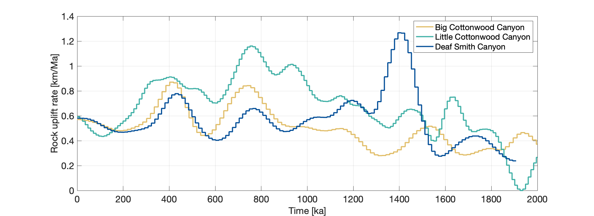
3.6. Rock uplift history of the Wasatch Fault
The extracted rock uplift rates are shown in figure 11. Over the last one million years, rock uplift rate histories derived from all three catchments record similar variations. Moving from the present back in time, there is an upturn towards the present beginning at approx. 150 ka. There are then two distinct peaks in rock uplift rate, one at approximately 400 ka, and another at approximately 750 ka. Beyond 1 Ma, the recovered rates become less correlated, likely due to the effects of geomorphic noise (see section 4.1). On longer wavelengths, there is an apparent increase in rock uplift rates from 2Ma to 1Ma. These results are discussed in detail in the following section.

4. Discussion
4.1. Knickzone production in the Wasatch
Knickzones are sections of a river network that have a different slope to the river network upstream and downstream. Knickzones can be produced by a variety of geological and geomorphic processes, which can have an influence on river network inversion results. Knickzone production in rivers has been attributed to lithological contacts (Allen et al., 2013; Wolpert & Forte, 2021), external forcing by tectonics, climate or base-level change (Leith et al., 2018; Petit et al., 2017; Whittaker & Boulton, 2012), and autogenic formation due to geomorphic feedbacks (Groh & Scheingross, 2021). The river networks examined in this study contain a series of knickzones that correspond to sections of high and low channel steepness index (fig. 4). In the downstream portions of the river network, these knickzones, representing high rock uplift rates, are correlated in our rock uplift rate histories (fig. 11). However, in the upstream portions that have older response times, the oscillations in rock uplift rate exhibit fewer correlations.
In the lower portion of the river networks, it is unlikely that lithological contacts, autogenic knickpoint production or base-level fall are responsible for knickzone production. On lithology, each network incises different bedrock lithologies, and the knickzones do not correlate to lithological contacts (Bryant, 2003; fig. 4). It is also unlikely that autogenic knickpoint production, which is dependent on factors such as sediment supply and lithology, could create similarly spaced knickpoints in all three of our geologically different catchments. Furthermore, autogenic knickpoint production refers to the creation of much smaller, evenly spaced vertical-step knickpoints or waterfalls (Groh & Scheingross, 2021), as opposed to the slope-break knickpoints observed in these catchments. Finally, we would not expect base-level fall to significantly influence this setting as the base-level is set by the Wasatch Fault. Although in the past, pluvial lakes may have raised the base-level above the fault, as the river profile is already graded to the Wasatch Fault, this only has the effect of shortening the river profile. When the lake level and base-level falls, the profile should be able to return to a similar form as before providing it can efficiently incise through any sediment fill. In this way, the river profile is unlikely to change steepness significantly as a result of lake filling and infilling influencing base level. What is more likely, is that the downstream knickpoints formed as a result of changes in climatic or tectonic regimes. A discussion of which is more likely is provided in the next section, and the supplementary material.
In the upper portion of the river networks, the tectonic signal imprinted into the network by the Wasatch Fault has had longer to become masked by other geomorphic processes. For example, in the upstream portions of Big Cottonwood Canyon, beaver dams have created flat sections of the river, and in Little Cottonwood Canyon, landslides at Tanner’s gulch are responsible for steepening the river downstream (fig. 4). This emphasizes our focus on the rock uplift rate history derived from the downstream portion of the river profiles.
4.2. Constraining Erodibility
Calibration of the inferred rock uplift rate history is performed by finding the K value that causes the amount of rock uplift derived from the river network to match that of an independent geological measurement of rock uplift/erosion (Fox et al., 2014; Goren et al., 2014; McNab et al., 2018; Pritchard et al., 2009; Racano et al., 2021). In previous studies, a single estimated value of K is used to recover rock uplift rates for all rivers in the inversion, which can span regions on the 1000 km2 scale (Goren et al., 2014; Racano et al., 2021), up to the continental scale (Roberts et al., 2012; Roberts & White, 2010).
Our methodology differs from these previous studies in that we allow K to be different in different catchments, despite the relatively small (< 500 km2) area they cover. This is because the river networks in this study incise different lithologies, and we expect that this will influence erodibility. We have shown that bedrock strength in these catchments differs significantly, and that calibrating the inversions to minimize misfit between rock uplift rate histories suggests using different K values between catchments is appropriate. However, we can also interrogate an erosion rate data set derived from 10Be cosmogenic nuclides (Stock et al., 2009) and erodibility estimates using the method of Goren (2016) to further constrain expected differences.
4.2.1. Erodibility from Erosion rate – ksn relationship
Our K values were inferred from the long term exhumation rate derived from thermochronometry, that we assume to be similar to the erosion rate (P. A. Armstrong et al., 2003; Ehlers et al., 2003). However, the time interval over which exhumation is recorded by the apatite (U-Th)/He system is larger than the time interval recorded by the lower portion of the river profiles in this study. It is thus possible that the exhumation rate experienced by the river profiles is different to that experienced by the thermochronometry samples. If this is the case, the estimated K values may be incorrect.
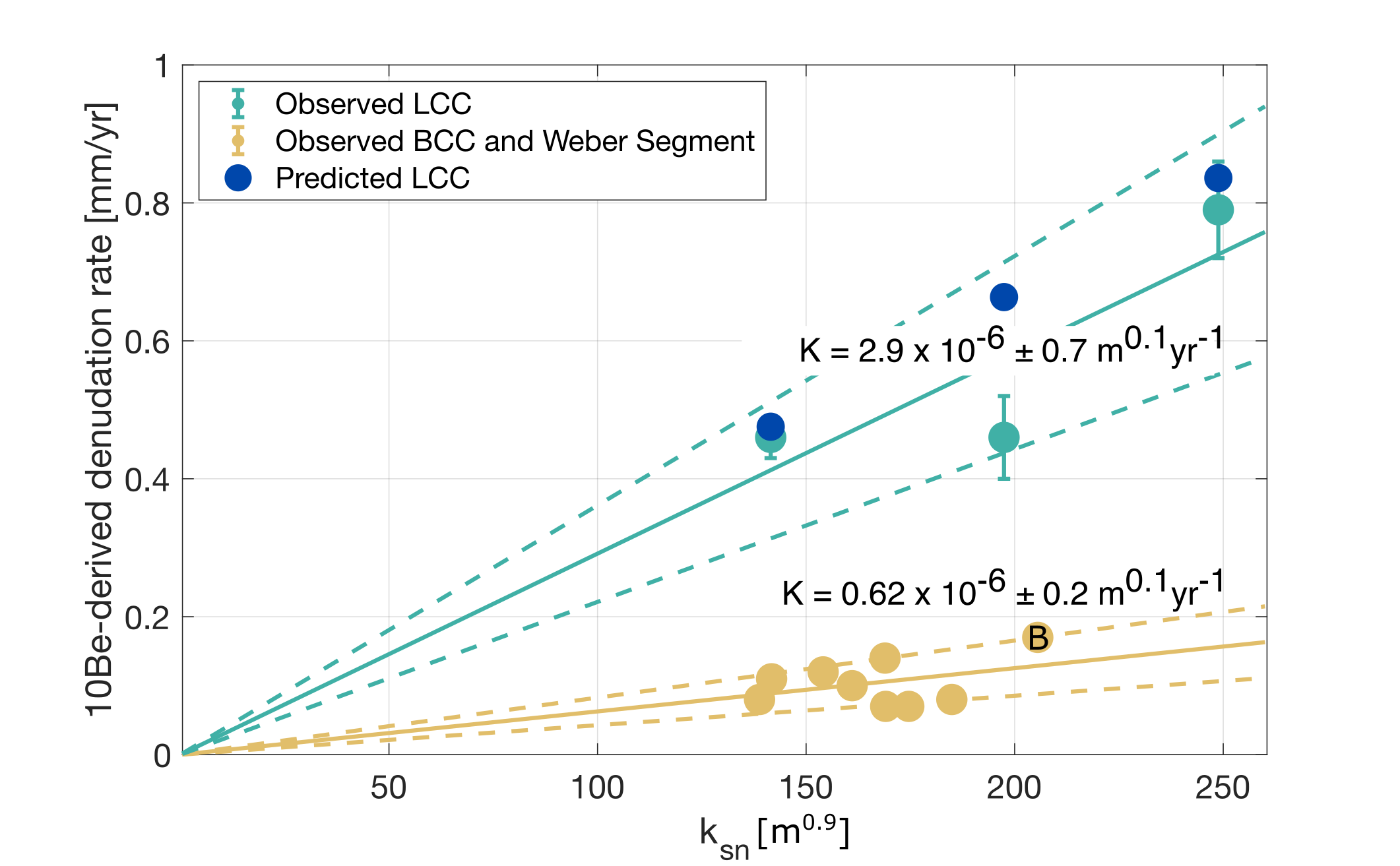
However, K can also be constrained from the erosion rate - channel steepness index relationship, as explained in section 2.5.3. Figure 12 shows catchment wide denudation rate derived from 10Be measurements vs catchment averaged channel steepness index for the catchments analyzed by Stock et al. (2009). The data set has been split into two groups; catchments from Little Cottonwood Canyon, and a catchment from Big Cottonwood Canyon plus Weber segment catchments which also erode quartizites, and schists and gneisses (Bryant, 2003; fig. 1). Some erosion rate - channel steepness index data sets exhibit non-linearity, and so it is necessary to fit a power law function through them. This has been used as evidence that the slope exponent, n, does not equal 1 (Adams et al., 2020; Gallen & Wegmann, 2017). In our study, there is insufficient coverage to derive n by fitting such a regression. The data set is thus used neither to argue linearity or non-linearity in the stream power model. Instead, we fit linear regressions through the two data sets, where the gradient of the lines represents the erodibility, K. This provides a simple constraint on the erodibility estimate.

Also plotted in figure 12 are predicted erosion rate - channel steepness index points for the catchments in Little Cottonwood Canyon for which there are cosmogenic 10Be measurements. These points represent erosion rates that have been calculated by multiplying the average channel steepness index of the catchment by the erodibility value inferred from our inversion calibration. This allows us to assess whether the erodibility used to derive long-term rock uplift rates is reasonable, compared to modern erosion rates.
There are two important findings that can be drawn from this data set. The first is that the erodibility value used in our inversion matches, within error, the erodibility derived from the short-term erosion rates. The significance of this is discussed in section 4.3. The second, is that the erodibility value predicted for Little Cottonwood Canyon catchments is 5 × greater than the erodibility value predicted for the Weber segment and Big Cottonwood Canyon catchments. Again, this provides support for the use of different erodibilities in the rock uplift rate calibration of each catchment, and that Little Cottonwood Canyon has a higher erodibility than the other catchments in this study. However, again there is a greater disparity between the erodibility values predicted from the 10Be erosion rate data set than the erodibility differences predicted by the inversion, and the Schmidt hammer and point load measurements. This disparity may be due to different bedrock lithologies of the Weber segment catchments (which erode Precambrian gneisses) but, could also be due to differences in climate owing to the distance between the Weber segment catchments and our study area, or errors associated with fitting a simple regression model. In any case, we predict distinct differences in the erodibility on short spatial scales but infer similar erodibility values from both the short-medium term erosion rate data from cosmogenic nuclides and the long-term rock uplift rate history derived from the river networks and calibrated using thermochronometry. This suggests that erodibility has been relatively constant through time.
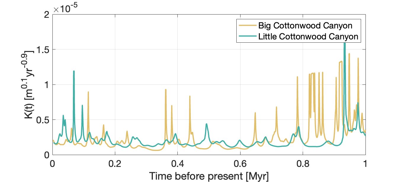
4.2.2. Erodibility through time
Our analysis assumes that the erodibility of the catchments is temporally invariant. To assess whether this assumption is appropriate, we must examine how lithology and climate may change through time. For catchments where rock units have different bedrock strengths, and are dipping sub-horizontally, erodibility may vary significantly through time, as the river network incises through different rock units (Gallen, 2018). For our catchments however, the effects of this are likely to be negligible as Little Cottonwood Canyon incises a granodiorite intrusion, and the sedimentary sequence in Big Cottonwood Canyon, and Deaf Smith Canyon is tilted sub-vertically, primarily to the NE, at 85° to 50°. This means that as the river networks incise, the boundary between the dominant units should not move significantly.
To investigate whether any other factors, such as climate, could influence erodibility through time, we use the methodology of Goren (2016), as detailed in section 2.6. This allows us to: a) assess whether erosion rate variation is driven either by changes in tectonics or erodibility, and b) further constrain the value of K.
The change in erodibility through time for Big and Little Cottonwood Canyon is shown in figure 13. The average inferred K value for Little Cottonwood Canyon over the 1 Ma time interval is 2.8 ×10⁻⁶ m0.1 yr−1, similar to that inferred from the cosmogenic data set (fig. 12) and the value inferred from our inversion calibration. We therefore believe that the K value for this catchment has been accurately inferred. Noise influences the K inference beyond 0.8 Ma in Big Cottonwood Canyon, but the average K value between 0 and 0.8 Ma for Big Cottonwood Canyon is 1.6 ×10⁻⁶ m0.1 yr−1, again lower than that predicted for Little Cottonwood Canyon, a trend consistent with predictions from our inversion results, Schmidt hammer and point load data, and the 10Be denudation rate data.
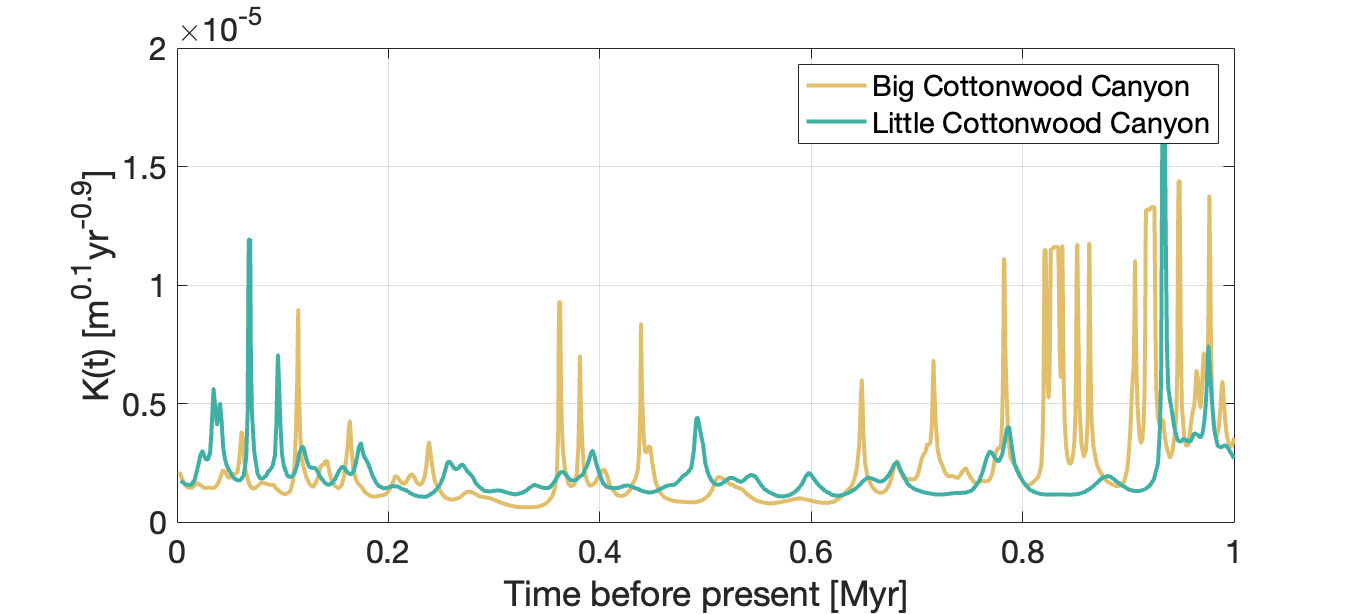
The observed changes in erodibility through time are different to the variation observed in rock uplift rate over the same time period. Variations have greater amplitudes and much shorter wavelengths, and do not seem to be correlated between catchments. Synthetic testing (supplementary material 1) shows that the spiky signal of erodibility recovered from this methodology is what would be expected if erodibility were constant through time, but rock uplift rate varied. The double peak signal recovered in the rock uplift rate histories of all three catchments is thus likely to be the result of tectonic changes.
4.3. Testing Linear Assumption
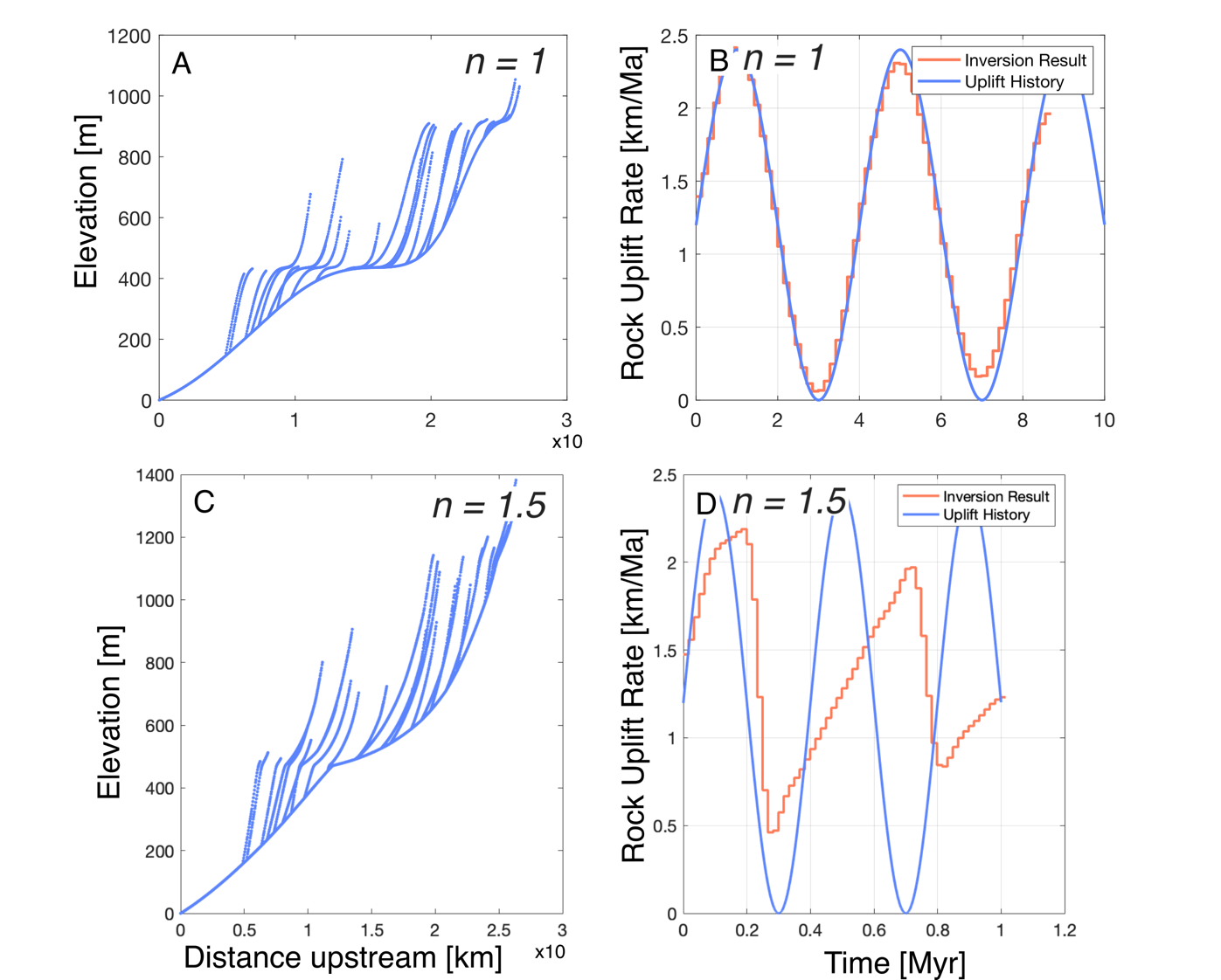
We use the analytical solution to the linear stream power model to infer the rock uplift rate history of the Wasatch. The methodology requires we make the assumption that, n, the slope exponent of the SPIM (Equation 2), is 1. However, the value of n is debated and predicted values span an order of magnitude between 0.7 (Whipple & Tucker, 1999) and 7 (Gallen & Fernández‐Blanco, 2021). In spite of this, the n = 1 assumption has been justified and evidenced in a variety of tectonic settings by different methodologies (Ferrier et al., 2013; Goren et al., 2014; Roberts et al., 2012; Schwanghart & Scherler, 2020; Wobus et al., 2006). Here, we demonstrate the effects of n being greater than one on linear river network inversions by simulating a river network using the FastScape algorithm (Braun & Willett, 2013), and show that the n = 1 assumption is valid for the Wasatch range by leveraging the calibration of the dimensionless rock uplift rate histories over different timescales.
We simulated two identical river networks using the FastScape algorithm, one under n = 1 conditions, and the other with n = 1.5. The profiles were created using an identical, oscillating rock uplift rate history, but different values for erodibility, so that the total elevation of the networks were comparable. We then invert the river network topography to recover the dimensionless rock uplift rate history (fig. 14). The rock uplift rate history is then calibrated so that the exhumation rate matches the average exhumation rate inputted into the FastScape algorithm.
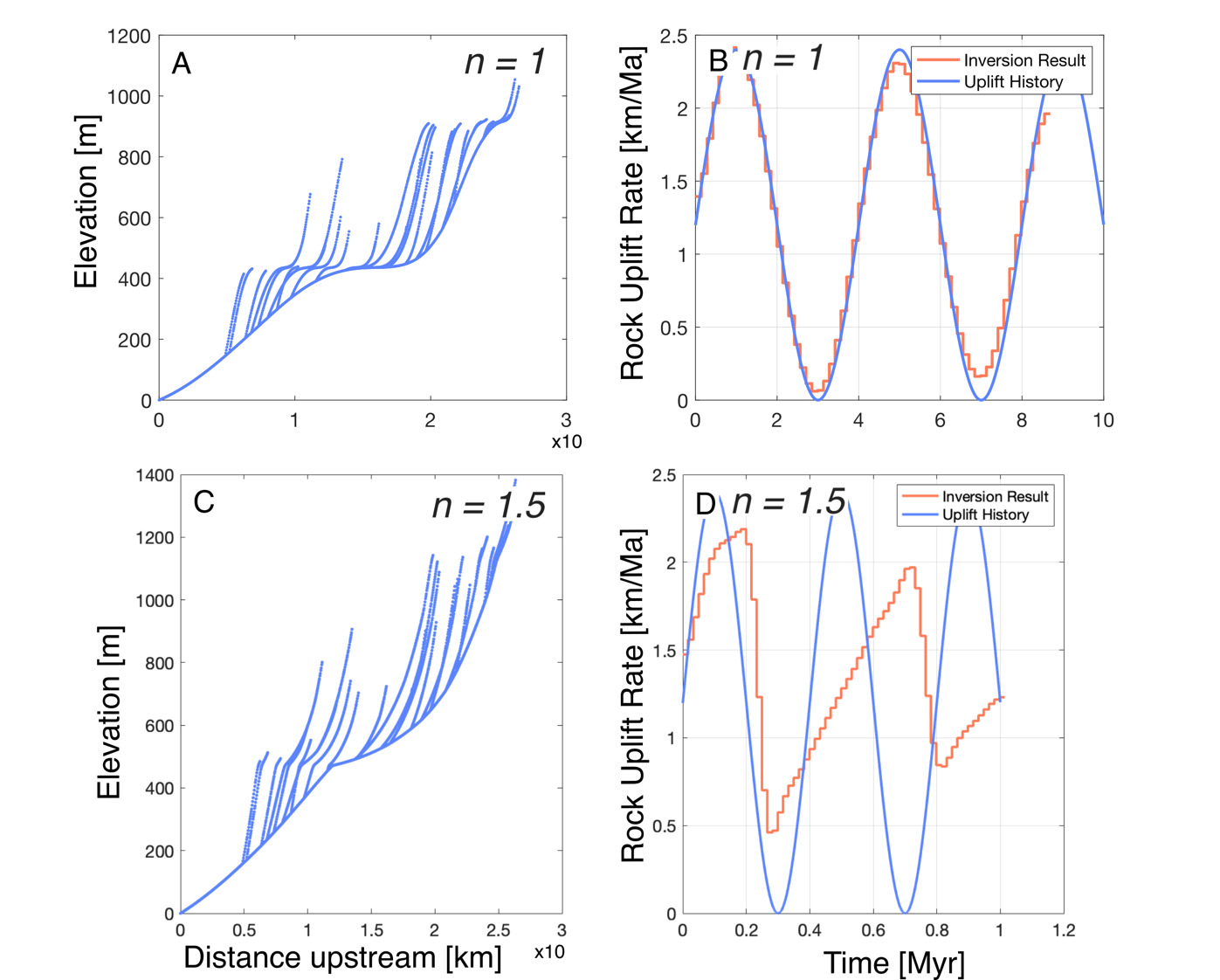
The consequence of the n being greater than 1 is that steeper channel segments propagate through a river network more quickly than flatter segments. For an inversion assuming n = 1, this can be problematic. Firstly, low uplift rate sections of the inferred history will be removed, which causes peaks in rock uplift rate to appear asymmetric (fig. 14). Note however that this is not the case in our inferred rock uplift rate histories (fig. 11). Secondly, when the uplift rate history is calibrated, the inferred rates will be lower than the actual rates to account for removal of low uplift rate sections. The predicted response time is therefore longer, meaning that changes in the rock uplift rate history will appear to occur further back in time. From figure 14, we can see that the more recent inferred rock uplift rate history is very similar to the input rock uplift rate history. However, as we infer further back in time, peaks of the inferred rock uplift rate history become smaller, more asymmetric and are predicted to occur at older time periods compared to the true peaks.
4.3.1. Is the n = 1 assumption valid for the Wasatch?
If n does not equal 1, there are important consequences for the inferred rock uplift rate history. However, we can show evidence that the value of n in the Wasatch is either 1, or close to 1, validating this assumption.
The calibration of inferred rock uplift rate histories requires knowledge of an independent geological constraint. However, the time over which the inferred history is matched can be different based on the constraint used. Short-medium term erosion rate data derived from cosmogenic 10Be spans the 103−104 year timescale, but thermochronometry records exhumation on the 106 −107 scale. A river network under n = 1 conditions preserves the entire rock uplift history experienced from the present to the maximum response time of the network. Therefore, regardless of the time interval over which rock uplift is measured, the correctly calibrated, inferred rock uplift rate will predict the same amount of rock uplift as the geological constraint. In other words, the K value needed to calibrate the inferred rock uplift rate history to both a short-term and long-term geological constraint will be similar (see fig. 14 B). However, if n is greater than 1, then parts of the rock uplift history are lost from the river network, as low slope sections are erased by downstream, higher slope sections that propagate more quickly through the network. Over short timescales, the rock uplift rate history captured by geological constraints and the inferred history will be similar (fig. 14D), as there has not been sufficient time for sections of the profile to be erased. However, on longer timescales portions of the river network representing slow periods of rock uplift have been lost. When the network is inverted, the amount of exhumation preserved in the river network is less than the amount of rock uplift rate recorded by a long-term geological constraint (e.g. thermochronology). To compensate for this, a greater value of K would be used in the calibration, which causes the calibrated rock uplift rates to be greater (eq 10), increasing the total amount of rock uplift rate preserved in the network. As a result, under n ≠ 1 conditions, the K value predicted from calibrating with a long term constraint will be smaller than the K value predicted from the short term constraint.
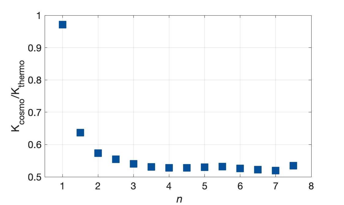
To investigate how different the predicted K values may be depending on the time interval over which the calibration is performed, we use a simple synthetic data set. We simulate a river profile using the FastScape algorithm for a range of values of n between 1 and 7. The rock uplift rate history used to produce the profiles oscillates, similar to that shown in figure 14. We then use the simulated profile elevations in a simple linear inversion to infer the dimensionless rock uplift rate history. The inferred rock uplift rate history is calibrated based on two different geological constraints; one at 30 000 years, and one at 1 million years, that are calculated directly from the input rock uplift rate history to the forward model. The dimensionless rock uplift rate is calibrated twice, by changing the K value so that the inferred rock uplift matches the rock uplift predicted by the short-term constraint, and then again so that it matches the rock uplift predicted by the long-term constraint. This gives two K values, representing calibration to both a short- and long-term constraint, for each simulated river profile produced for the given value of n. We determine the ratio between these two K values, and then plot this against the range of values of n (fig. 15), to show how different the K values might be for values of n greater than 1. We denote the K value derived from the calibration using the short-term constraint Kcosmo, and the K value derived from the calibration using the long term constraint Kthermo.

When n is 1, the values of K inferred from the short-term constraint and the long term constraint are similar, hence the value of Kcosmo/Kthermo is close to 1. However, there is a dramatic decrease in the value of this ratio when n is not 1. The K value determined from calibrating the river profile using an older constraint is lower than the K value determined from a short term constraint, which is consistent with the theoretical prediction above.
In the Wasatch, we have shown that the K value used to calibrate our rock uplift rate history is very similar to the K value predicted from the channel steepness index - erosion rate relationship (fig. 15). Our inferred K value from the calibration of river network inversions is based on a million year thermochronological constraint, whereas the K value inferred from the channel steepness index - erosion rate relationship is based on short-medium term cosmogenic 10Be data. Given that these K values show good agreement in our study and given the relationship between Kcosmo/Kthermo for different values of n (fig. 15), we expect the value of n in our study area to be 1 or very close to 1.
4.4. Climate driven rock uplift variation
The effects of loads on the Earth’s surface on slip rates of both normal and reverse faults has been well documented in a number of settings (Hampel et al., 2010; Johnston, 1987; Olive et al., 2014; Xue et al., 2022). In particular, lakes have been shown to have significant influence on slip rates on normal faults (Hampel et al., 2010; Hetzel & Hampel, 2005; Karow & Hampel, 2010; Xue et al., 2022), with studies linking this effect directly to the Wasatch Fault, albeit only for the most recent episode of deep lake filling associated with Lake Bonneville (Hampel et al., 2010; Hampel & Hetzel, 2006). Lake Bonneville covered a 52 000 km2 of the basin, and was deepest on the hanging wall of the Salt Lake City segment of the Wasatch Fault, reaching depths of 350 m (Austermann et al., 2020; Hampel et al., 2010; Oviatt & Jewell, 2016). Loading of the Wasatch Fault by Lake Bonneville suppressed slip for the period in which the deep lake was present, a phenomenon which has also been observed on other normal faults (Xue et al., 2022). This is because the Wasatch fault is a low-angle normal fault, and so increasing the vertical component of stress would increase the normal stress on the fault plane, locking it. Following a rapid reduction in the lake level, the fault is able to slip again, and studies have suggested that for the Wasatch Fault, slip rate doubles compared to the previous, pre-lake filling rate (Friedrich et al., 2003; Hampel et al., 2010; Hetzel & Hampel, 2005). It therefore stands to reason that during a cycle of deep lake filling and emptying, we would expect to see coeval changes in rock uplift rate on the fault.
Lake filling in the Bonneville Basin occurs during glacial periods, where precipitation increases and evaporation decreases (Belanger et al., 2022). Lake filling initiated in the Bonneville Basin sometime between 760 and 600 ka (Davis, 1998), and the largest lakes formed during the most extreme glacial periods: deep lake deposits are dated at 420 ka, 150 ka and 28–12 ka (Oviatt et al., 1999).
Our inversion results show three distinct increases in rock uplift rate on the Wasatch Fault recorded by all three catchments in the last million years. These occur at approximately 750–700 ka, 450–400 ka and 150–0 ka (fig. 11). These peaks occur, within error, during time periods when the deepest lakes were present in the Bonneville basin (see the supplementary material for further discussion). Given that the most recent lake, Lake Bonneville, has been shown to cause increases in rock uplift rate, we suggest that the increases in rock uplift rate recovered in our inversion are similarly related to lake filling and emptying. The implication is that climate change has indirectly affected rock uplift rates on the Wasatch Fault over the past 800 ka due to the presence of pluvial lakes. Further implications exist for assessing seismic hazard in the region, for which increased seismicity is already observed during dry periods (Young et al., 2021), as the present day Great Salt Lake continues to recede due to ongoing drought in the region.
5. Conclusions
We present a robust rock uplift rate history for the Salt Lake City Segment of the Wasatch Fault between 1 Ma to the present derived from analysis of river networks. We use a number of data sets and methodologies to validate our methodology and our recovered rock uplift rate history. We show that differences in erodibility between two of the river networks, predicted from both our inversion, and a previously published cosmogenic 10Be erosion rate data set, can be linked to differences in lithology. This is assessed with Schmidt hammer and point load rock strength measurements. Combining these data sets with our inversion of fluvial topography allows us to investigate the controls on erodibility. We find that erodibility is not controlled by bedrock strength alone, but rather the contrast between the bedrock and bedload strength. Having shown that erodibility is variable in space, we then show that erodibility is relatively invariant through time using the approach Goren (2016) and comparison of the erodibility value inferred from the inversion, with that derived from the cosmogenic 10Be data set. This gives good confidence that our recovered variations in rock uplift rate are indeed driven by tectonic forcing, and not changes in erodibility through time.
We also show that in the Wasatch, the slope exponent of the SPIM, n, is likely to be close to 1. This is evidenced by the similarity of the erodibility predicted from the calibration of the dimensionless rock uplift rate over the long term, and the erodibility calculated from the erosion rate data set. If n were greater than 1, we would not expect these values to be so similar, given the loss of information the river network experiences in these conditions.
Finally, the rock uplift rate histories inferred from all three river networks show two distinct peaks in rock uplift at approximately 700 ka and 400 ka, and an upturn between 150 ka and the present. These periods coincide with deep lake formation in the Bonneville basin. Previous studies have shown that Lake Bonneville filling and emptying has caused changes in rock uplift rate on the Wasatch Fault, but for the first time we show evidence that this phenomenon has repeated over the past 800 ka. Our result provides evidence for climate change indirectly influencing tectonics, with implications for our understanding of fault behavior throughout the glacial-interglacial cycles of the Pleistocene.
Acknowledgments
We would like to thank Brendon Quirk for performing the point load testing, and Gerald Roberts and Anke Friedrich for insightful discussion that helped to improve this research. We would also like to thank reviewers Fiona Clubb and Frank Pazzaglia for insightful, constructive reviews that helped improve the manuscript. AS is supported by the Natural Environment Research Council [NE/S007229/1]. MF is supported by the Natural Environment Research Council [NE/N015479/1].
Author Contributions
AS Conceptualisation, Methodology, Data Curation, Formal Analysis, Writing - Original Draft. MF Conceptualisation, Methodology, Data Curation, Supervision, Writing - review and edits. JM Data Curation, Writing - review and edits. SM Data Curation, Writing - review and edits. LG Methodology, Writing - review and edits. MM Data Curation, Writing - review and edits. AC Conceptualisation, Supervision, Writing - review and edits.
Supplementary Data
https://doi.org/10.17632/dx2yjgm92h.1
Editor: Mark Brandon