Isotope Ratio – Discharge Relationships of Solutes Derived From Weathering Reactions

1. Introduction

The flux of rock-derived solutes in river networks reflects an integrated signature of the water-mineral-life interactions that drive chemical weathering in the critical zone. This flux is responsible for a significant component of total landscape denudation (Anderson, 2012; Hilley et al., 2010; Millot et al., 2002; Riebe et al., 2004; West et al., 2005), contributes to the global cycling of elements from the terrestrial environment to the oceans (Dupré et al., 2003; White & Blum, 1995), and functions as a principal regulator of atmospheric carbon (Hilton & West, 2020; Jepsen et al., 2016). Thus, a wealth of vital information is contained within the dissolved solute content and composition of fluvial systems (e.g., Bouchez & Gaillardet, 2014; Gaillardet et al., 1999; Torres et al., 2015). However, these data are complicated by the rate at which water drains through landscapes, which varies widely both in space (e.g., heterogeneous permeability, slope, flow path) and in time (e.g., wet vs. dry seasons, evapotranspiration, snowmelt). Thus, solute concentrations ($C$) are often cast as a function of the discharge rate (Q) of the fluvial system, resulting in delineation of distinct concentration-discharge ($C$-Q) patterns including mobilization, dilution and chemostasis (Godsey et al., 2009; Ibarra et al., 2017; Knapp et al., 2020; Maher, 2010, 2011). Within this long-term behavior, higher temporal resolution observations reflect distinct and repeatable patterns even at a single sampling point. Both seasonal and event-based observations show that the rising and falling limbs of the hydrograph reflect unique solute concentrations, resulting in hysteresis loops in the $C$-Q response to storm events (Arora et al., 2020; Knapp et al., 2022; Rose et al., 2018; Winnick et al., 2017; Wymore et al., 2019). The nuances of this integrated watershed signal clearly hold a wealth of information reflecting both the (bio)geochemical structure and (bio)hydrologic plumbing of the critical zone, yet such data are only now beginning to be disentangled beyond the restrictive (and often invalid) assumptions of steady state infiltration and drainage.

1.1. Water-rock reactions and stable isotope ratios

The variety and relative pace of water-rock-life reactions that commonly take place in the near surface environment (Brantley, 2008; Brantley & White, 2009; White & Brantley, 2003) impart chemical signatures to the fluid draining through these landscapes which are recorded in the $C$-Q relationships of streams and rivers. In the simplest condition, primary minerals (e.g., the minerals composing unweathered bedrock) are dissolved by infiltrating, weakly acidic rainwater, releasing solutes into solution. Under this condition, one may reasonably infer that if a sufficiently slow flow rate is maintained, the solute concentrations will plateau at the maximum values achievable between the lithology of the system and the infiltrating fluid prior to discharge (Ameli et al., 2017; Maher, 2010, 2011). However, most major ions are heavily influenced by a combination of primary mineral dissolution and the precipitation of secondary phases favored to form under ambient, near-surface conditions (Brantley & White, 2009; Chorover et al., 2007). In addition, many elements which have been dissolved into solution become further cycled by vegetation through the critical zone (Bouchez & von Blanckenburg, 2021; Frings, Oelze, et al., 2021; Frings, Schubring, et al., 2021). Thus, in natural environments, both the magnitude of solute concentrations and the appearance of a maximum or plateau reflect a balance between increasing concentrations due to dissolution of some phases, decreasing concentrations due to formation of new secondary solids and biological activity and the influence of common ion effects on solubility. Further, periods of quiescence interspersed by infiltration events create the potential for transient fluid saturation states, and even the capacity to re-dissolve secondary phases (Dellinger et al., 2015), which further complicates interpretation.

Stated equivalently, a series of N reactive pathways, each following a linear and reversible TST-type rate expression through time $(t)$:

$$\begin{aligned} \frac{dC}{dt} &= k_{1}\left( 1 - \frac{C}{C_{\text{lim1}}} \right) + k_{2}\left( 1 - \frac{C}{C_{\text{lim2}}} \right)\ldots\\ & \qquad + k_{N}\left( 1 - \frac{C}{C_{\text{limN}}} \right)\\ &= \sum_{i = 1}^{N}{k_{i}\left( 1 - \frac{C}{C_{lim_{i}}} \right)} \end{aligned}\tag{1}$$

can be solved for the initial condition $C = C_{0}$ at $t = 0$ and cast as an effective or cumulative single reactive pathway by introducing terms $k_{eff} = \sum_{i}^{}k_{i}$ and $C_\text{LIM} = \left( \sum_{i}^{}k_{i} \right)\text{/}\sum_{i}^{}\left( k_{i}\text{/}C_{lim_{i}} \right)$ (see Supplementary Section S1 for a full demonstration of this equivalency), yielding:

$$C(t) = C_{\text{LIM}} + \left( C_{0} - C_{\text{LIM}} \right)\,\exp{\left( - \frac{k_{eff}}{C_{LIM}}t \right)\tag{2}}$$

Here $C_{\text{LIM}}$ is the maximum concentration of a given element or compound in solution that the parcel of fluid can reach and $k_{eff}$ is a kinetic rate constant with units of concentration per time. The term $C_{\text{LIM}}$ is essentially an equivalent limiting concentration that is weighted by the individual limiting concentrations and the individual reaction rate constants ($k_{i}$; Supplementary Information S1). We emphasize the use of $C_{\text{LIM}}$ rather than the stricter equilibrium $C_{eq}$ in reference to the simplified behavior of this single component system and the potential combination of multiple individual $C_{lim_{i}}$ to produce an effective maximum for a given solute in a given system. The under-constrained nature of the problem is highlighted by equation (2) in that an intractable variety of primary mineral dissolution and secondary mineral formation pathways may produce equivalent values of $C$, $k_{eff}$ and $C_{\text{LIM}}$ .

The stable isotope signatures of these solutes offer a means of disentangling equation (2) and more complex multi-component systems. Mass-dependent fractionation is commonly minimal if not absent when bedrock is dissolved by reactive fluids (Brantley et al., 2004; Hellmann et al., 2012; Oelkers, 2001), leading to the inheritance of the solid phase isotope ratio in the dissolved load. In contrast, both formation of new secondary phases and biological cycling commonly exert mass-bias, leading to a characteristic shift in the isotope ratios of the solutes that remain in the fluid (Fernandez et al., 2019; Gabitov et al., 2012; Geilert et al., 2014; Mavromatis et al., 2013; Oelze et al., 2015; Rustad et al., 2010; Tang et al., 2008; Watkins et al., 2013). This identifying signature of a subclass of reactive pathways is the vital constraint that stable isotope ratios afford in the study of critical zone weathering (Bouchez et al., 2013) and allows us to reframe equation (2) to parse between two categories of reactions: those that are fractionating and those that are not.

To date, most isotopic analyses of geogenic solutes in fluvial systems have focused on large rivers over long timescales (Baronas et al., 2018; Charbonnier et al., 2020; Dellinger et al., 2015; Frings et al., 2016; Henchiri et al., 2016; Pogge von Strandmann & Henderson, 2015). A growing number of studies are beginning to report the riverine signatures of stable isotope ratios in the major elements participating in weathering reactions at sufficient spatiotemporal resolution to consider their relationship to $C$-Q patterns in watersheds (Engström et al., 2010; Fernandez et al., 2022; Georg et al., 2006; Golla et al., 2022; Pokrovsky et al., 2013; Riotte et al., 2018). However, interpretation has largely been restricted to mixing models or simplified approximations of transient hydrologic behavior.

1.2. Fluid residence time and storage functions

Water-rock-life reactions that produce a given solute concentration are often subject to kinetic constraints and are hence tightly coupled to fluid age (i.e., the time elapsed since water was introduced) in the near-surface critical zone (Rinaldo & Marani, 1987). Natural subsurface environments are heterogeneous, such that packets of fluid infiltrating into the soil will travel through an ensemble of pathways characterized by different lengths and velocities, leading to a distribution of fluid residence times. This coupling of reactivity to fluid age distributions was described in a series of seminal studies by Maher (2010, 2011) for the chemical weathering of a silicate mineral assemblage. Maher (2010, 2011) used typical functional forms for the age distribution of fluid in watersheds, which are generally skewed towards younger water but feature a long ‘tail’ of older water contributions. Using this class of fluid age distributions, Maher (2010, 2011) showed that the integrated signature of a solute derived from weathering reactions would appear lower or less reacted than in a system where all water is the same age. Building on this basis, Torres and Baronas (2021) expanded the same modeling approach to explicitly consider both dissolution of primary minerals and precipitation of secondary phases.

These models offer a vital link between the range of fluid ages a watershed can host and the manifestation of flux-weighted solute concentrations as observed in streams and rivers. However, they did not address the variability of fluid transit times that are expected and widely observed during individual storm events. The ubiquity of hysteresis relationships such as those described above highlights the importance of input chronology in critical zone systems. In reality, flowpaths are not a fixed property of the landscape as they typically follow cycles of activity/inactivity depending on soil moisture content and water table elevation (Dralle et al., 2018; McGlynn et al., 2004; Tetzlaff et al., 2007; Tromp-van Meerveld & McDonnell, 2006; Zimmer et al., 2013). This triggers a substantial time-variance in subsurface residence time distributions and results in streamflow age that varies continuously as a function of hydrologic response. A typical result is that the share of younger water in streamflow increases during high flows, due to the activation of faster pathways that provide younger water. If we think of water age as a metric for the contact time between the fluid and the minerals which compose near-surface structure, the variability in streamflow age is a relevant element to explore $C$-Q relationships (Benettin, Bailey, et al., 2017). Further, this history of water residence and associated solute concentration is not encapsulated by ensemble averages of multiple fluid transit times from stationary models. Such need to account for the time-variability of streamflow age thus inspired the formulation of transport based on ‘StorAge Selection’ (SAS) functions (Botter et al., 2011). From this perspective it is difficult to imagine a system that returns precisely the same concentration of solute for a given discharge rate through all time, even if the $C$-Q relationship falls within the operational definition of chemostasis. Presently, the use of stationary transit time distributions in models for $C$-Q behavior does not encapsulate this linkage to the history of hydrologic forcing preserved in the fluids stored by watersheds.

1.3. Toward isotope ratio-discharge relationships

The power-law framework commonly utilized to interpret $C$-Q behavior embeds the effects of dilution as a principle means of producing negative slopes in $C$-Q space (Godsey et al., 2009; Musolff et al., 2015). The stable isotope ratios of dissolved solutes, once corrected for atmospheric inputs, should not be directly impacted by dilution. Hence the idea of a complementary “$\delta$-Q” relationship may appear irrational. However, given the sensitivity of stable isotope ratios to a subset of common weathering reactions (section 1.1), we may anticipate that low-order catchments subject to dynamic precipitation events should routinely produce transient shifts in mineral saturation state, periods of heightened or diminished secondary mineral formation / primary mineral dissolution and even re-dissolution of secondary phases, leading to a predictive relationship between riverine isotope ratios, discharge, and the history of water stored in the system. Thus, dynamic $\delta$-Q relationships (e.g., hysteresis patterns) should reflect subsurface reactivity (Fernandez et al., 2022; Golla et al., 2022) and should be largely spared from the compounding effects of direct dilution in the fluvial drainage network.

Based on this rich potential for advancement using a combination of $C$-$\delta$-Q patterns, we present the first development of a model that embeds stable isotope fractionation and transient flow dynamics. A new model package is produced and openly distributed with this updated functionality, and we present a series of demonstrations increasing in complexity from a batch reactor advancing through time to a realistic watershed structure and precipitation record. In doing so, the present study addresses the following guiding questions:

1. Do variable fluid storage ages produce isotopic hysteresis?

2. Do differences in event history produce characteristic patterns in $\delta$-Q?

3. Is there a direct relationship between isotope ratios and the age of water discharging from the critical zone?

Finally, we demonstrate a comparison of our model results to a new compilation of silicon isotope ratios in six low-order streams subject to transient storm events (Fernandez et al., 2022). Through development and distribution of this new model package it is our intention to offer a timely complement to the emerging wealth of riverine weathering isotope datasets that are now being produced at increasingly high temporal resolutions.

2. Model Development

2.1. Transient water age distributions

Unlike laboratory batch experiments, watersheds contain, and rivers aggregate a distribution of past rainfall events (McGuire & McDonnell, 2006). Thus, streamflow has a distribution of water ages that range from ‘young’ water (recent rainfall events) to ‘old’ water (rainfall from previous years). These distributions are generally expected to vary over time (Botter et al., 2010) because flowpath velocity and activation are strongly dependent on storage dynamics, leading to the general expectation of larger shares of young water in streamflow during wet periods. To deal with time-varying water age distributions, we use a lumped parameter model based on StorAge Selection (SAS) functions (Botter et al., 2011; Harman, 2015; van der Velde et al., 2012). The SAS approach was specifically developed to deal with time-variable transit time distributions and is based on the so-called ‘water age balance equation’, which is a water balance applied separately to each individual water parcel (see Supplementary Section S2). To solve the water age balance, one needs to prescribe a SAS function Ω [-], which quantifies the rates at which stored parcels are exported to the stream (similar to an age-specific mortality rate in demography). A complete description of the SAS approach would be lengthy and beyond the scope of the present work, but extensive details and formulas can be found in the recent review paper by Benettin et al. (2022). Here, we use a power SAS function (Queloz et al., 2015) of the type

$$\Omega\left( S_{T},t \right) = \left\lbrack \frac{S_{T}(T,t)}{S_{0} + V(t)} \right\rbrack^{z(t)}\tag{3}$$

where $S_{0}$ is the initial water storage, T is the age of the water, i.e., the time elapsed since it entered the system, V(t) is the relative water storage computed by solving the water balance and z > 0 is a distribution parameter. Equation (3) is a unitless probability density function defined over a finite support [0, 1]. We chose the power function because it has less parameters than other distributions (like the beta) and because it already proved successful in simulating water age dynamics in real-world watersheds (e.g., Grandi & Bertuzzo, 2022; Lapides et al., 2022; Sprenger et al., 2022; Zhang et al., 2021). The exponent z can be interpreted as a “shape” parameter that controls the shape of the age distribution and the term $S_{0}$ can be seen as a “scale” parameter that controls the temporal scale. The water in rivers is known to be, on average, younger than the water storage that the river drains (Berghuijs & Kirchner, 2017) and this translates into a parameter z < 1. However, it is reasonable to expect more marked contributions of young water when a catchment is wetter (Benettin et al., 2022; Harman, 2015). Therefore, similar to previous applications in watersheds (Benettin et al., 2020; Visser et al., 2019; Wilusz et al., 2017), we allow the exponent z to vary over time, with lower/higher values under wetter/drier periods (see numerical implementation in Section 2.4). Once the parameters of the SAS function are given and the water age balance is solved to give the rank storage S_T (T, t), the transient water age distributions can be computed as:

$$p_{Q}(T,t) = \frac{\partial\Omega_{Q}\left( S_{T},t \right)}{\partial S_{T}}\frac{\partial S_{T}}{\partial T}\tag{4}$$

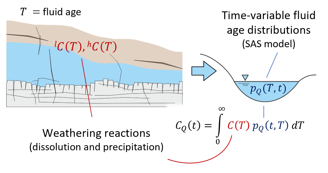
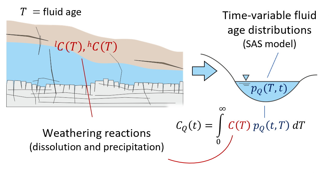
Following the notation of equations (1–2), we indicate $C(T)$ as the concentration of a reactive tracer after a residence time $T$. The tracer concentration in streamflow $(C_{Q})$ is then computed by integrating the tracer contribution of all the fluid parcels of different ages that contribute to streamflow (convolution integral):

$$C_{Q}(t) = \int_{0}^{\infty}{C(T)}\, p_{Q}(T,t)\, dT\tag{5}$$

equation (5), either with time-variables or fixed age distributions, is used in the reminder of the paper to simulate streamflow tracer concentration and isotope ratios.

We note that the SAS function approach used here employs a single storage volume encapsulating the time-variable range of fluid ages within (and discharging from) the system. By combining such a model with a set of water-rock reactions, we are essentially aggregating all reactivity into one representative parameterization including time-invariant rate constants, solubility limits and mineral reactive surface areas. This allows us to model the evolution of solute chemistry over a range of times based on our time-varying fluid ages, but it inherently compromises resolution of mineralogical heterogeneity within the near-surface environment. Furthermore, we omit direct representation of common ion effects that will arise as a result of shifts in multi-component solute chemistry, in keeping with the approach of Maher (2010, 2011), Ibarra et al. (2017), and Torres and Baronas (2021). These simplifications are introduced to isolate the effects of non-stationarity in the water age distribution on the resulting aqueous chemical composition and stable isotope ratio of a homogeneous storage volume (fig. 1).

2.2. Stable isotope fractionation of a solute subject to weathering reactions

We first require that the concentration $C$ of a given solute as shown in equation (2) is comprised of two isotopes, ^h$C$ and ^l$C$, where ^h$C$ + ^l$C$ = $C$. This notation is used to refer to a heavy (h) and light (l) mass, e.g., ³⁰Si and ²⁸Si, ⁷Li and ⁶Li, ⁴⁴Ca and ⁴⁰Ca. These two isotopes of $C$ are subject to the same set of reactions:

$$\frac{d^{l}C}{dT} = {{ }^{l}{k}}_{eff}^{}\left( 1 - \frac{{{ }^{l}C}^{}}{{ }^{l}C_{LIM}^{}} \right)\tag{6}$$

$$\frac{d^{h}C}{dT} = {{ }^{h}{k}}_{eff}^{}\left( 1 - \frac{{ }^{h}C}{{ }^{h}C_{LIM}^{}} \right)\tag{7}$$

with nominally equivalent values of $k_{eff}$ and values of $C_{lim}$ that are distinguished by the relative abundance of the two isotopes comprising the overall concentration $C$. The ratio of the two is then typically defined as

$$r = \frac{{ }^{h}C}{{ }^{l}C}\tag{8}$$

critically, some of the individual reactions (eq 1) that are embedded within the equivalent overall reaction (eq 2) may support slight mass-dependent differences in the rate at which the reaction proceeds, leading to shifts or ‘fractionation’ in the ratio of the two isotopes

$$\alpha_{i} = \frac{{{ }^{h}{k}}_{i}^{}}{{{ }^{l}{k}}_{i}^{}}\tag{9}$$

When $\alpha_i$ is 1.0, the individual reaction does not impart kinetic fractionation.

The key inference here is that some of the individual reactions embedded in equation (6–7) may fractionate the isotopic ratios (eq 9) between the fluid and solid phase(s), while others do not. This leads us to distinguish two subgroups within the overall effective reaction rate expression for each isotope, those that are fractionating and those that are not.

$$\frac{d{ }^{l}C}{dT} = {{ }^{l}{k}}_{1}^{}\left( 1 - \frac{{ }^{l}C}{{ }^{l}C_{LIM1}^{}} \right) + {{ }^{l}{k}}_{2}^{}\left( 1 - \frac{{ }^{l}C}{{ }^{l}C_{LIM2}^{}} \right)\tag{10}$$

$$\begin{aligned} \frac{d{ }^{h}C}{dT} &= {{ }^{h}{k}}_{1}^{}\left( 1 - \frac{{ }^{h}C}{{ }^{h}C_{LIM1}^{}} \right)\\ & \quad + {{ }^{h}{k}}_{2}^{}\left( 1 - \frac{{ }^{h}C}{{ }^{h}C_{LIM2}^{}} \right)\\ & =\alpha_1{ }^l k_1\left(1-\frac{r^l C}{r_{L I M 1}{ }^l C_{L I M 1}}\right)\\ & \quad +\alpha_2{ }^l k_2\left(1-\frac{r^l C}{r_{L I M 2}{ }^l C_{L I M 2}}\right) \end{aligned}\tag{11}$$

Where $\alpha_{1}$ = 1.0 and thus “group 1” is composed of individual reactions that are non-fractionating, while $\alpha_{2}$ ≠ 1.0 represents a net effective fractionation factor for “group 2”, i.e., those reactions that do impart fractionation due to fluid-rock-life interactions. As noted in equation (11), the definitions of $\alpha$ and $r$ allow us to write both rate expressions using the same kinetic rate constants and limiting concentrations, a convention that is typical in the development of isotopic rate expressions (DePaolo, 2011).

Fortunately, this expansion of a classic linear reversible rate expression can still produce a closed form analytical solution (see Section S3 for full derivation). The solution to this ordinary differential equation yields explicit expressions for ${ }^{l}C$ and ${ }^{h}C$ as a function of time:

$$\begin{aligned} { }^{l}C(T) &= { }^{l}C_{LIM}^{}\\ & \quad + \left({ }^{l}C_{0}^{} -{ }^{l}C_{LIM}^{} \right)\, e^{- \left( \frac{k_{1}}{{ }^{l}C_{lim1}^{}} + \frac{k_{2}}{{ }^{l}C_{lim2}^{}} \right)\, T} \end{aligned}\tag{12}$$

$$\begin{aligned} { }^{h}C(T) &= { }^{h}C_{LIM}^{}\\ & \quad + \left({ }^{h}C_{0}^{} -{ }^{h}C_{LIM}^{} \right)\, e^{- \left( \frac{k_{1}}{{ }^{h}C_{lim1}^{}} + \frac{k_{2}}{{ }^{h}C_{lim2}^{}} \right)\, T}\\ &= { }^* C_{L I M}\\ & \quad +\left(r_0 { }^l C_0 - { }^*C_{L I M} \right) e^{-\left(\frac{\alpha_1 k_1}{r_{l i m 1}{ }^l C_{l i m 1}}+\frac{\alpha_2 k_2}{r_{l i m 2}{ }^l C_{l i m 2}}\right) T} \end{aligned}\tag{13}$$

where ${C}_{0}$ is the concentration at T = 0 and ${ }^* C_{L I M} = \left( \sum_{i}^{}\alpha_{i}k_{i} \right)\text{/}\sum_{i}^{}\left( \alpha_{i}k_{i}\text{/}\left( r_{lim_{i}}{{ }^{l}C}_{lim_{i}}^{} \right) \right)$.

Assuming the component of the reaction rate belonging to group 1 (i.e., ${k}_1$(1 −$C$/$C_{lim_{1}}$)) is associated with the higher value of $C_{lim}$ and hence will always be dissolving and non-fractionating, the value of ${r}_{lim_{1}}$ may be set equal to an appropriate value to reflect the bedrock primary mineral assemblage. This means that the contribution of group 1 to the overall reaction rate will be to increase $C$ and shift the fluid isotope ratio towards a bedrock value. If group 2 (i.e., ${k}_2$(1 − $C$/$C_{lim_{2}}$)) is fractionating ($\alpha_2$ ≠ 1.0) then a simple expectation would be that this component of the overall reaction exhibits classic distillation as the system proceeds towards $C_{lim_{2}}$. This is easily implemented in equation $(13)$ by setting the value of ${r}_{lim_{2}}$ to the instantaneous isotope ratio of the fluid phase at any given time (t) over the course of reaction progress. Unfortunately, this does cause equation $(13)$ to become implicit, but with sufficiently high-resolution time steps (i.e., much smaller than the characteristic time scale of the reaction) the value of ${r}_{lim_{2}}$ at the previous time step functions appropriately for this purpose. In doing so, the fractionation factor associated with the group 2 component of the reaction rate is a constant and equal to $\alpha_2$ at all times. Finally, we accommodate an important caveat in equation (13), recognizing that any given reactive pathway in this system is reversible, but dissolution of a solid phase is typically associated with minimal to negligible fractionation, whereas precipitation exhibits mass-dependent bias. Thus, we require that for any $\alpha_2$ ≠ 1.0, this effect is only imparted when the solubility is such that the system is growing new mineral rather than (re)dissolving it. To ensure this important feature we make the restriction that

$$\small{\alpha_{2} = \left\{ \begin{array}{r} \neq 1.0\ if\ \left({ }^{l}C +{ }^{h}C \right) > \left({ }^{l}C_{LIM2}^{} +{ }^{h}C_{LIM2}^{} \right) \\ = 1.0\ if\ \left({ }^{l}C +{ }^{h}C \right) \leq \left({ }^{l}C_{LIM2}^{} +{ }^{h}C_{LIM2}^{} \right) \end{array} \right.}\tag{14}$$

The approach described above is straightforward in that we can always recover Rayleigh distillation by simplifying the system such that ${k}_1 = 0$ and $C_0 > C_{lim_{2}}$, thus providing an important basis for expected behavior in the model (see Section S3 for demonstration). Further, this approach is consistent with the interpretation of many fractionating reactions in application to critical zone studies (Bouchez et al., 2013; von Blanckenburg & Schuessler, 2014).

Thus far we have presented the adaptation of a set of linear reversible rate expressions to accommodate stable isotope fractionation in a relatively generic format that could be applied to a variety of stable isotope systems. In application to the stable isotope ratios typically utilized to track the weathering and vegetation cycling origins of riverine solutes, we would reasonably specify a non-unity value for $\alpha_2$ that is slightly less that 1.0, e.g., ~0.998 for $\delta$³⁰Si (Fernandez et al., 2019; Geilert et al., 2014; Oelze et al., 2015) or ~0.988 for $\delta$⁷Li (Golla et al., 2021). Similarly, we would reasonably set ${r}_{LIM1}$ to a ratio typical of the natural abundance of these isotopes in primary mineral assemblages, such that the value in delta notation would be ~0.00‰. Finally, we may reasonably choose an ${r}_{LIM2}$ that is slightly negative in delta notation, e.g. −1.00‰ for $\delta$³⁰Si or −10.0‰ for $\delta$⁷Li, to represent the signatures of secondary minerals (e.g., clays) that have accumulated in the weathering profile. Though beyond the scope of this work, we acknowledge that mineral-specific isotope compositions within a given bedrock assemblage have been observed and may offer an additional source of (generally minor) variations in fluid isotope ratios during dissolution.

The basic functioning of the model is now described (sections 2.1 and 2.2) and illustrated schematically in figure 1.

Figure 1.Schematic illustration of the model summarizing governing equations. Transient water age distributions (eq 4) are combined with a set of first-order kinetic rate laws (eqs 12 and 13) using a convolution integral (eq 5) to yield time-dependent streamflow solute concentrations and isotope ratios.

2.3. Water-rock reactions

We next require a representative set of water-rock reactions typical of silicate weathering in Critical Zone systems. The present model is somewhat unique in that we do not wish to summarize the entire set of weathering reactions into one representative rate law (e.g., Lebedeva et al., 2007; Lebedeva & Brantley, 2013) but, given the lumped volume hydrologic model, we also do not wish to turn to a full multi-component numerical reactive transport model (e.g., Ackerer et al., 2021; Golla et al., 2021; Heidari et al., 2017; L. Li et al., 2007; Maher et al., 2009; Navarre-Sitchler et al., 2009; Perez-Fodich & Derry, 2019). Instead, we wish to partition two classes of reactions, those that only dissolve minerals into solution (i.e., irreversible), and those that are capable of both dissolution and precipitation (i.e., reversible; eqs 10 and 11). In this respect the present model parameterization requirements are similar to a recent study by Torres and Baronas (2021), who also partitioned an overall weathering reaction into dissolution and precipitation components in their treatment of dissolved silicon. As they noted, there exists substantial ambiguity in the relative rates of primary mineral dissolution and secondary clay precipitation. Many studies suggest rate constants for clays that are orders of magnitude lower than those for primary mineral dissolution, yet these clays exhibit characteristically high surface areas, which produce overall rates that can vary widely between locations and in comparison between laboratory and field-derived observations. Given this ambiguity, we follow the approach adopted by Torres and Baronas (2021) and utilize a ratio of net precipitation rate to dissolution rate $(R_{p}/R_{d})$ that encompasses both rate constants and reactive surface areas and falls between values of 0.1–1.0. This range is narrower than the parameter space Torres & Baronas (2021) tested through Monte-Carlo sampling, and reflects the general expectation that clay formation rates are somewhat slower than primary mineral dissolution rates. We demonstrate several specific values of $(R_{p}/R_{d})$ (fig. S3) and elect to conduct the majority of our simulations using a value of 0.5, which is consistent with the ratio suggested by Maher (2011) as appropriate for the contemporaneous dissolution of albite and accumulation of kaolinite.

Unlike the Torres and Baronas (2021) study, we do not work in normalized ratios of the $C_{lim_{i}}$ values, but rather allow the fractionating component of the overall reaction to remove solute from solution only when $C_{lim_{2}}$ is exceeded. To estimate these values, we turn to a previously developed multi-component silicate mineral weathering model built in the open-source software CrunchFlow (Maher et al., 2009). This simulation was validated against mineralogy and aqueous chemistry depth profiles across a chronosequence of marine terraces near Santa Cruz, California, USA and a similar simplification of this model served as the basis for parameterization of Maher (2010, 2011). The same model was later extended to consider the influence of organic acids on mineral weathering rates (Lawrence et al., 2014) and most recently the storage and isotopic composition of soil carbon (Druhan & Lawrence, 2021). For the present purpose, this CrunchFlow model simply offers a well constrained and robust basis to extract representative values of $C_{lim_{i}}$ if (1) only primary minerals are included (i.e., group 1) and (2) if only secondary clays are considered (i.e., group 2). For our group 1 reactions we extract a maximum $\text{SiO}_{2(\text{aq})}$ concentration of 800 µM and set this equal to $C_{lim_{1}}$. For our group 2 reactions, we similarly reach a maximum $\text{SiO}_{2(\text{aq})}$ concentration of 150 µM and set this equal to $C_{lim_{2}}$ (see Supplementary Section S4 for numerical modeling details). Importantly, the kinetic parameters and mineral surface areas used in these prior models (Supplementary Information S3, S4) are only indirectly incorporated into the present study. Essentially, we rely on the rigorous thermodynamics and stoichiometry developed in these prior data-validated multi-component numerical simulations to produce appropriate values of $C_{lim}$ for our present purposes and proceed by utilizing these values in combination with an appropriate representation of $R_{p}/R_{d}$. This combination of parameter values derived from a realistic silicate weathering reaction network in combination with our range of $R_{p}/R_{d}$ values produces a system in which clays feature a lower solubility threshold than a contemporaneous assemblage of primary minerals, and these clays generally react slightly slower than the feldspars.

Many possible combinations of rate constants (encapsulating both intrinsic constants and mineral surface areas) could be chosen such that a specific $R_{p}/R_{d}$ ratio may be achieved. However, in combination with our limiting concentrations ($C_{lim_{1}}$ = 800 µM and $C_{lim_{2}}$ = 150 µM), we may utilize the relationship $C_{LIM} = \left( \sum_{i}^{}k_{i} \right)\text{/}\sum_{i}^{}\left( k_{i}\text{/}C_{lim_{i}} \right)$ used to recast equation (1) into equation (2) to ensure values of ${k}_{i}$ that produce an overall $C_{lim}$ that is consistent with observations and prior models. For example, $R_{p}/R_{d}$ = 0.5 may be achieved by using ${k}_1$ = 1µM/day and ${k}_2$ = 0.5µM/day, such that we produce a $C_{LIM}$ = 327µM with a characteristic timescale of 218 days. This timescale and maximum concentration are both consistent with the models developed by Maher (2010, 2011) for $\text{SiO}_{2(\text{aq})}$ solute dynamics (see Section S5 for demonstration). Further in keeping with Maher (2010, 2011) and Torres and Baronas (2021), from this point forward, the remainder of the models are presented in terms of dissolved $\text{SiO}_{2(\text{aq})}$ and hence an appropriate fractionation factor of $\alpha_2$ = 0.998 is applied (Fernandez et al., 2019; Frings, Oelze, et al., 2021; Geilert et al., 2014). However, we emphasize that this in no way limits the present model development to the Si system, simply that appropriate parameter representations are necessary to treat a given solute with this basic model framework.

2.4. Numerical implementation

The test hydrologic dataset consists of synthetically generated input (rainfall) and output (streamflow) data. Rainfall was generated at a daily scale as a Poisson process with annual rainfall depth of 1200 mm and mean inter-arrival of 10 days. This relatively large inter-arrival was selected to minimize overlapping events. Rainfall was then uniformly downscaled to hourly resolution. For the sake of simplicity, we neglected any evaporative and deep losses. The runoff response was modeled through two non-linear bucket models (see e.g., Kirchner, 2016b), which can be interpreted as a soil and a groundwater system. The outflow from the soil system partly forms direct runoff $({Q}_{s})$ and partly recharges the groundwater system. All groundwater outflow is assumed to flow into the stream as groundwater flow $({Q}_{gw})$. This type of lumped 2-box model is an established approach to generate realistic runoff responses. Similar to Harman (2015) and Benettin, Soulsby et al. (2017) we define a metric of catchment wetness (w(t)) to control the variability of the SAS function (eq $3$), by letting the SAS parameter z vary linearly between a minimum value (z_min) during wettest periods (w = 1) and a maximum value (z_max) during driest periods (w = 0):

$$z(t) = z_{\min} + \left( 1 - w(t) \right)\,\left( z_{\max} - z_{\min} \right)\tag{15}$$

The variable w can be defined in many ways based on observational data (soil moisture or runoff) or modeled data. Since we generated the hydrologic data, we defined w(t) as the ratio of soil versus total runoff $w=Q_s /\left(Q_s+Q_{g w}\right)$ (additional details can be found in Supplementary Section S6 and figure S3).

We implemented the chemical equations (12–13) into a new version of the tran-SAS package (Benettin & Bertuzzo, 2018), which is made publicly available under the name tran-SAS_Weathering (Benettin & Druhan, 2023). All the results presented in this paper are generated (and are reproducible) through this model. We solved the water age balance using a Euler Forward solution at 3-hour timesteps, which guarantees sufficient numerical accuracy while keeping computational times short. The model was run over 8 years, where the first 6 years were used as spinup and the last 2 years were kept for analysis. The spinup is necessary to populate the water storage with a large number of new water parcels and we selected 6 years because it is much larger (about 10 times) than the characteristic timescale of the reaction. The water age component of the model makes use of 3 parameters ($S_{0}$, ${z}_{min}$, ${z}_{max}$, as defined in eqs 3 and 15). These are initially kept fixed (reference value) and then two additional sets of parameters are subsequently tested to characterize distinct transport behaviors and water age dynamics. Set 1 is representative of a small hydrologic system (small water storage) that always releases relatively younger water to streamflow. Set 2 represents a much larger hydrologic volume with more extreme variations in streamflow age, switching from young water release during wet periods to old water release during very dry periods. These parameter sets are selected to highlight two key aspects of the transport process: the timescale (reflected in the storage parameter) and the sensitivity to water flux variability (reflected in the ${z}_{min}$–${z}_{max}$ range). The parameter values are plausible and similar to values identified in real-world catchments in previous studies (Benettin, Bailey, et al., 2017; Benettin, Soulsby, et al., 2017; Grandi & Bertuzzo, 2022). The chemical parameters were kept the same throughout the paper, as given in table 1.

The model outputs include solute concentration, isotope ratios and water age distributions. To characterize the time-variability of water age distributions, we computed the young water fraction F_yw (Kirchner, 2016a) for different age threshold τ_yw. F_yw quantifies the fraction of streamflow that is younger than τ_yw and thus it is confined within the interval (0, 1). For example, a value of F₁₀ = 0.3 means that 30% of streamflow is made of water younger than 10 days, while the rest is older. We selected 4 values of τ_yw: 14 days, to quantify the fraction of very young water; 75 days, which is the standard value (between 3 and 4 months) used in the literature (see Kirchner, 2016a); 218 days, which is the temporal scale of the effective kinetic constant ${k}_{eff}$; and finally 352 days, obtained as the previous threshold plus the time needed by the reaction to reach $C_{lim_{2}}$, which is also representative of an annual timescale.

3. Results

3.1 Batch and stationary fluid age distributions

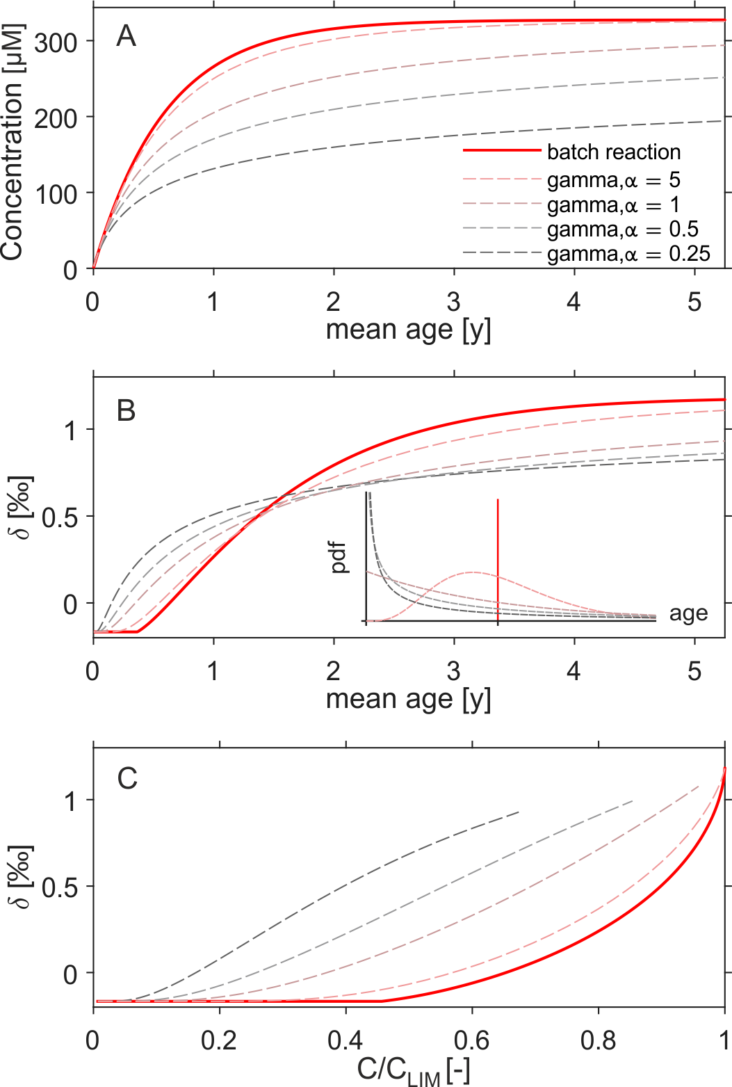
The silicate weathering model described in subsections 2.2–2.3 is first demonstrated in a simplified system in which fluid $\text{SiO}_{2(\text{aq})}$ concentrations are allowed to evolve from an initial value of zero at a water age of zero to a final steady state $C_{LIM}$ as the age of the fluid advances (fig. 2A, red line). Rate constants of ${k}_1$ = 1 µM/d and ${k}_2$ = 0.5 µM/d yield an $(R_{p}/R_{d})$ = 0.5 and result in a $C_{LIM}$ = 327 µM which agrees very closely with the prior Maher (2010, 2011) model (Supplemental Information figure S2). This close agreement lends further support to the validity of our model behavior, both in the $C_{LIM}$ steady state concentration and in the timescale over which this value is achieved. However, it is vital to understand that the present model establishes comparable results through the combination of two representative reactive pathways with unique rate constants and solubility limits, as opposed to the earlier Maher (2010, 2011) approach, in which a single ${C}_{eq}$ value is employed. Furthermore, the model remains single-component, omitting the influence of common-ion effects and generally producing relatively slower temporal evolution of the fluid isotope ratios than comparable multi-component geochemical models (Winnick et al., 2022).

Figure 2.(A) $\mathbf{SiO_{2(aq)}}$ concentrations increasing through time following the same parameters as the R_p/R_d = 0.5 simulation shown in Supplementary Information (solid red line). The concentrations from four representative gamma fluid age distributions with shape parameters of 0.25, 0.5, 1.0 and 5.0 are plotted in dashed lines. Mean fluid ages are calculated as the weighted average of each gamma distribution, and mean solute concentrations are calculated using eq 5 for each distribution, where the shape factor of 5.0 lies closest to the uniform simulation (red) and the shape factor of 0.25 is the furthest in comparison. (B) corresponding aqueous $\delta$³⁰Si time series. The inset further illustrates the gamma distribution shapes used in the computations (the mean value is the same for all and indicated with a vertical red line). (C) $\delta$³⁰Si vs. reaction progression from an initial condition ($C$/${C}_{LIM}$ = 0) to steady state ($C$/${C}_{LIM}$ = 1).

From this basis, we relax the assumption of a single uniform fluid age which advanced through time from an initial condition to a steady state $\text{SiO}_{2(\text{aq})}$ concentration. As we turn toward more realistic descriptions of watersheds, we begin with the behavior of this model convolved with relatively simple static fluid age distributions commonly used to represent an ensemble of flow paths through upland hill slopes. We choose four gamma distributions (shown in figure 2B inset) distinguished by their shape factors (5.0, 1.0, 0.5, 0.25) and convolve them with equation (12) to produce flux-weighted $\text{SiO}_{2(\text{aq})}$ concentrations and mean fluid ages that may be plotted in direct comparison to the batch results (fig. 2A). Two of these shape factors (0.5 and 0.25) were also used in Maher (2011) and continue to closely agree with the earlier study. As discussed by Maher (2011) and Maher and Chamberlain (2014), a smaller shape factor leads to a lower weighted average $\text{SiO}_{2(\text{aq})}$ concentration and hence the appearance of a lower effective reaction rate, despite consistency in the geochemical model parameters across all simulations. Higher shape factors produce a narrower range of fluid age distributions and hence a closer approximation of the batch model.

The use of two distinct reactive pathways allows us to implement stable isotope fractionation in the same modeling framework (fig. 2B & 2C). For parameters appropriate to describe $\delta$³⁰Si partitioning during silicate weathering (Section 1) the model achieves an enrichment in the fluid phase on the order of 1.20 as the system reaches steady state for an $(R_{p}/R_{d})$ = 0.5 (fig. 2B, red line). Here a subtle behavior of the isotope simulations is noted. At early time, specifically before the fluid $\text{SiO}_{2(\text{aq})}$ concentration has crossed the $C_{lim_{2}}$ threshold (eqs 12 and 13), both the primary mineral assemblage and the clays are dissolving and contributing to the increase in $\text{SiO}_{2(\text{aq})}$. As a result, the corresponding $\delta$³⁰Si value is a balance between primary minerals (group 1), specified as 0.00 ‰ and secondary clays (group 2), specified as -0.50 ‰ (table 1; Section 2.2). Once the $C_{lim_{2}}$ threshold is crossed, the “clay component” or group 2 of the reaction is now removing $\text{SiO}_{2(\text{aq})}$ from solution, while the primary mineral or group 1 component continues to dissolve. At this point, fractionation associated with the growth of new secondary clays occurs. Hence there is a period of time (or a range of fluid ages) for which no fractionating reactions influence Si.

Extending this simulated fluid $\delta$³⁰Si enrichment through time to a series of gamma distributions for fluid age creates distinctions in behavior relative to the batch model that are even more pronounced than those produced for $\text{SiO}_{2(\text{aq})}$ (fig. 2B). Even at early time, when the $\text{SiO}_{2(\text{aq})}$ concentrations of the batch model are less than $C_{lim_{2}}$ and hence there is no kinetic isotope fractionation, convolution of equations 12 and 13 with the gamma distributions returns $\delta$³⁰Si values that are enriched relative to the starting value. This is due to the effects of the tail in the gamma distributions, which produce a small component of the fluid that is already of sufficient age to cross the $C_{lim_{2}}$ threshold even when the mean fluid age is still lower than this value. The result is a recognition of the fact that any fluid age distribution that features even a minor component of ‘old’ water will incorporate some extent of fractionation associated with secondary mineral formation and hence enrichment in the fluid $\delta$³⁰Si values relative to that of a single age model. As time advances, the effect of these gamma distributions produces the appearance of muted reaction progress in the $\text{SiO}_{2(\text{aq})}$ concentrations (fig. 2A), and an associated dampening in the isotopic enrichment of fluid $\delta$³⁰Si (fig. 2B), though the effect is less pronounced than in the bulk solute concentrations. This behavior is closely tied to the enhanced enrichment in $\delta$³⁰Si for distributions with young mean fluid ages, where a lower shape factor creates a larger increase in $\delta$³⁰Si earlier in the simulation, and hence the muting of this isotopic enrichment as the mean fluid ages of the distributions increase is not as pronounced as it would be without this effect. The result is a crossover in the relationship between a batch model and the gamma age distributions in $\delta$³⁰Si space. For our parameter set, this crossover occurs at approximately 1.75 years, and is largely a function of the relative difference between the $C_{lim_{2}}$ and $C_{LIM}$ values.

Finally, comparison of the batch model results with the weighted $\text{SiO}_{2(\text{aq})}$ concentrations and $\delta$³⁰Si values is cast in terms of reaction progress from our initial condition of $\text{SiO}_{2(\text{aq})}$ = 0 to steady state (fig. 2C). For all choices of shape factor, the gamma distributions produce the appearance of greater fractionation in the fluid for a given point in reaction progress relative to the batch model. This is again a result of the strong effects of the tail in the gamma distribution, which produces a small but influential component of much older water and hence advanced reaction progress relative to a batch model. The result is that this restriction to fractionation only after the $C_{lim_{2}}$ threshold is crossed (eq 14) in combination with a component of older fluid ages in the gamma distributions could easily lead to the misinterpretation of fractionation factors if figure 2C were measured directly from samples taken in natural environmental system(s).

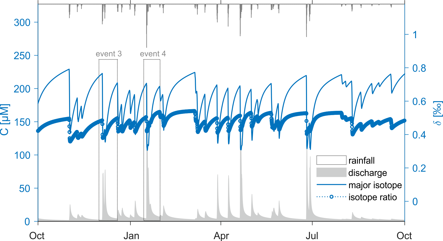
3.2. Time-varying fluid age distributions

From this basis we are poised to merge the fractionating weathering reactions developed in sections 2.2–2.3 with a SAS-function model incorporating time-varying fluid age distributions. We do so using a synthetic dataset, allowing the system to spin up over several years before focusing on a two-year period and a selection of individual rainfall-runoff events. Figure 3 illustrates the simulations over a 12-months interval. During this time, the specific hydrologic parameters and synthetic discharge record used to create a representative watershed produce $\text{SiO}_{2(\text{aq})}$ concentrations that range between 100 and 250 µM. Importantly, this means that the system is poised around the $C_{lim_{2}}$ = 150 µM threshold, such that some component of the fluid is likely to be undersaturated with respect to group 2 (the secondary clays) while another older component should be forming clays and hence driving isotopic fractionation. This is exhibited in the corresponding fluid $\delta$³⁰Si ratios, which fall in a relatively narrow range (0.35 to 0.55 ‰) of enrichment relative to the primary minerals and clay values (0.00 and -0.50 ‰, respectively, table 1). The concentration changes are rather sharp because the water age distributions change quickly at the onset of the hydrologic response.

Figure 3.One of the two years of simulation of a representative watershed using synthetic data. Discharge values are provided (grey shading) for the complete timeseries in addition to flux-weighted $\mathbf{SiO_{2(aq)}}$ concentrations (line) and fluid $\delta$³⁰Si ratios (dots).

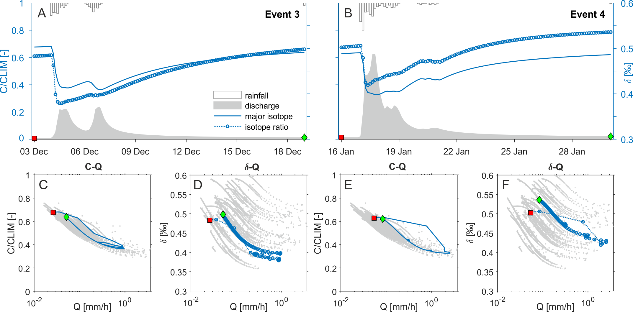
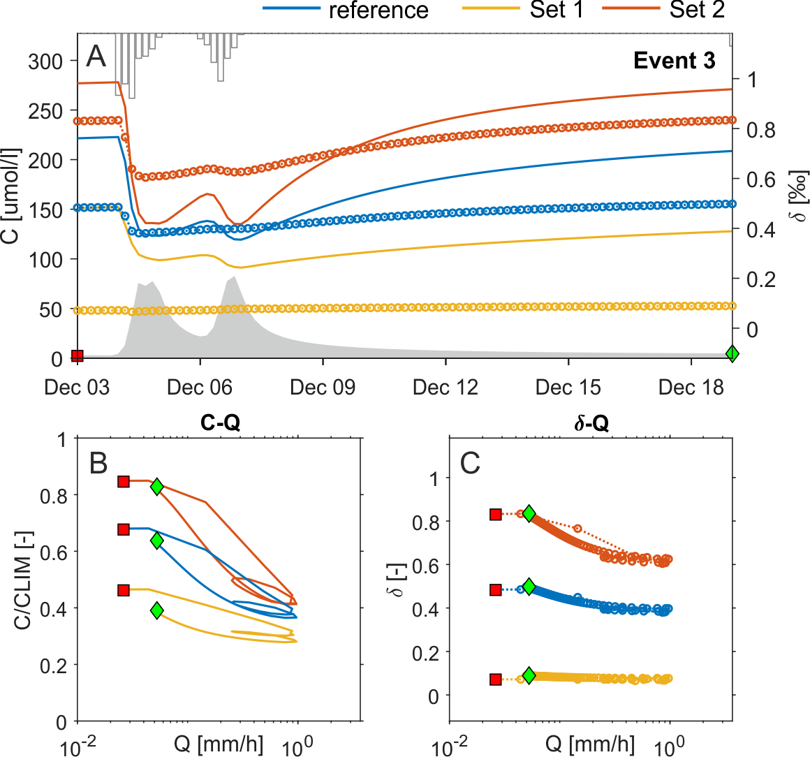
We choose two individual high-discharge events (hereafter termed Event 3 and Event 4) from this larger dataset (fig. 3) to explore in detail. The same analysis is provided for three additional events (Event 1, 2 and 5) in Supplementary Information figure S4. These events are not picked for any specific characteristics, but simply to display the variety of behavior that can be generated in both $\text{SiO}_{2(\text{aq})}$ and $\delta$³⁰Si in a single system for a single set of reactive parameters as a result of realistic time-varying hydrologic conditions. Event 3 (fig. 4A, C, D) is the first significant discharge event to occur after a relatively long period of quiescence, and it also features a double peak in the hydrograph over the course of approximately three days. Event 4 (fig. 4B, E, F) is comparatively larger, with a clear peak discharge value and a receding limb that lasts for several days after.

Figure 4.Two selected periods of high discharge: (A) after a relatively quiet interval and (B) during a relatively active interval of rainfall events. Event discharge values are plotted along the lower axis, while event precipitation is plotted along the upper axis. $\mathbf{SiO_{2(aq)}}$ and $\delta$³⁰Si are shown with a simple line and open circles, respectively. (C) the corresponding $\mathbf{SiO_{2(aq)}}$ vs. discharge (Q) relationship for the first event, (D) $\delta$³⁰Si vs. Q for the first event, (E) $\mathbf{SiO_{2(aq)}}$ vs. Q for the second event and (F) $\delta$³⁰Si vs. Q for the second event. A red square indicates the start of each event in time, while a green diamond reflects the end of this high discharge period. These markers highlight the directionality of hysteresis loops which emerge from the dataset. In panels C–F grey points reflect the entire synthetic dataset collected over the two-year period.

The double peak in discharge featured in Event 3 results in a somewhat complex hysteresis pattern in $\text{SiO}_{2(\text{aq})}$ vs. Q (fig. 4C) where the overall clockwise pattern is punctuated by a second smaller loop at the highest range of discharge values. The corresponding $\delta$³⁰Si vs. Q behavior (fig. 4D) shows a distinct behavior, in which the $\delta$³⁰Si values initially drop as Q increases to the lowest isotopic ratios recorded during this event, then slightly rebound during the period between the two discharge peaks, and ultimately recover to pre-event conditions. The result is a hysteresis loop that actually appears to rotate counterclockwise due to the overlapping of these multiple high discharge periods.

The much larger discharge values recorded in Event 4 cause a stronger clockwise hysteresis pattern in $\text{SiO}_{2(\text{aq})}$ vs. Q (fig. 4E) which reaches large values in comparison to the bulk of the dataset. The loop is also more consistent than that of Event 3, owing to the lack of such a pronounced double peak in discharge. The corresponding $\delta$³⁰Si vs. Q behavior (fig. 4F) also shows a larger hysteretic effect, this time creating the appearance of a clockwise pattern.

In both selected events, the weighted average $\text{SiO}_{2(\text{aq})}$ concentrations fall below 150 µM ($C_{lim_{2}}$) at peak discharge, yet at no time do the corresponding weighted average $\delta$³⁰Si values approach the bedrock $\delta$³⁰Si = 0.00 ‰. In fact, the second event appears to generate a longer period of time in which the $\text{SiO}_{2(\text{aq})}$ concentration remains below 150 µM and yet the overall range of $\delta$³⁰Si values is higher than that observed in the first event. This behavior underscores the importance of the fluid age distributions which underlie these calculations, as well as the importance of prior events in dictating current observations.

4. Discussion

4.1. The relationship between isotopic enrichment and water age

Coupling a SAS-function model to isotopically fractionating weathering reactions produces hysteresis patterns in the isotopic ratios of a reactive solute as a function of discharge over the course of a precipitation event (fig. 4). However, these loops are not as consistent in shape or even rotational direction as their solute counterparts. Irregular and even counterclockwise hysteresis patterns have previously been suggested in trace element ratios tracking silicate weathering (Kurtz et al., 2002), though the underlying causes have remained unclear. To our knowledge this model is the first to generate transient coupled $C$-Q and $\delta$-Q relationships from a forward mathematical framework.

Analysis of a selection of individual discharge events (fig. 4) suggests that a single reaction parameter set applied to a unique hydrologic system can produce a variety of $\delta$-Q patterns as a result of the characteristics of the individual event and the timing and duration of the events which preceded it. Across all events, both $\text{SiO}_{2(\text{aq})}$ and $\delta$³⁰Si values strongly respond to the initiation of a high discharge period (fig. 4A & B), yet the corresponding recovery to pre-event values appears to be faster in the isotope ratios relative to bulk solute concentrations. In the two events analyzed in section 3.2, the fluid $\delta$³⁰Si ratios reached values even higher than pre-event conditions over a period of time in which $\text{SiO}_{2(\text{aq})}$ had not fully recovered. This disparity in behavior suggests a distinct relationship between the fluid age distribution and the associated isotopic ratios, rather than simply a mirroring of the solute–fluid age relationship.

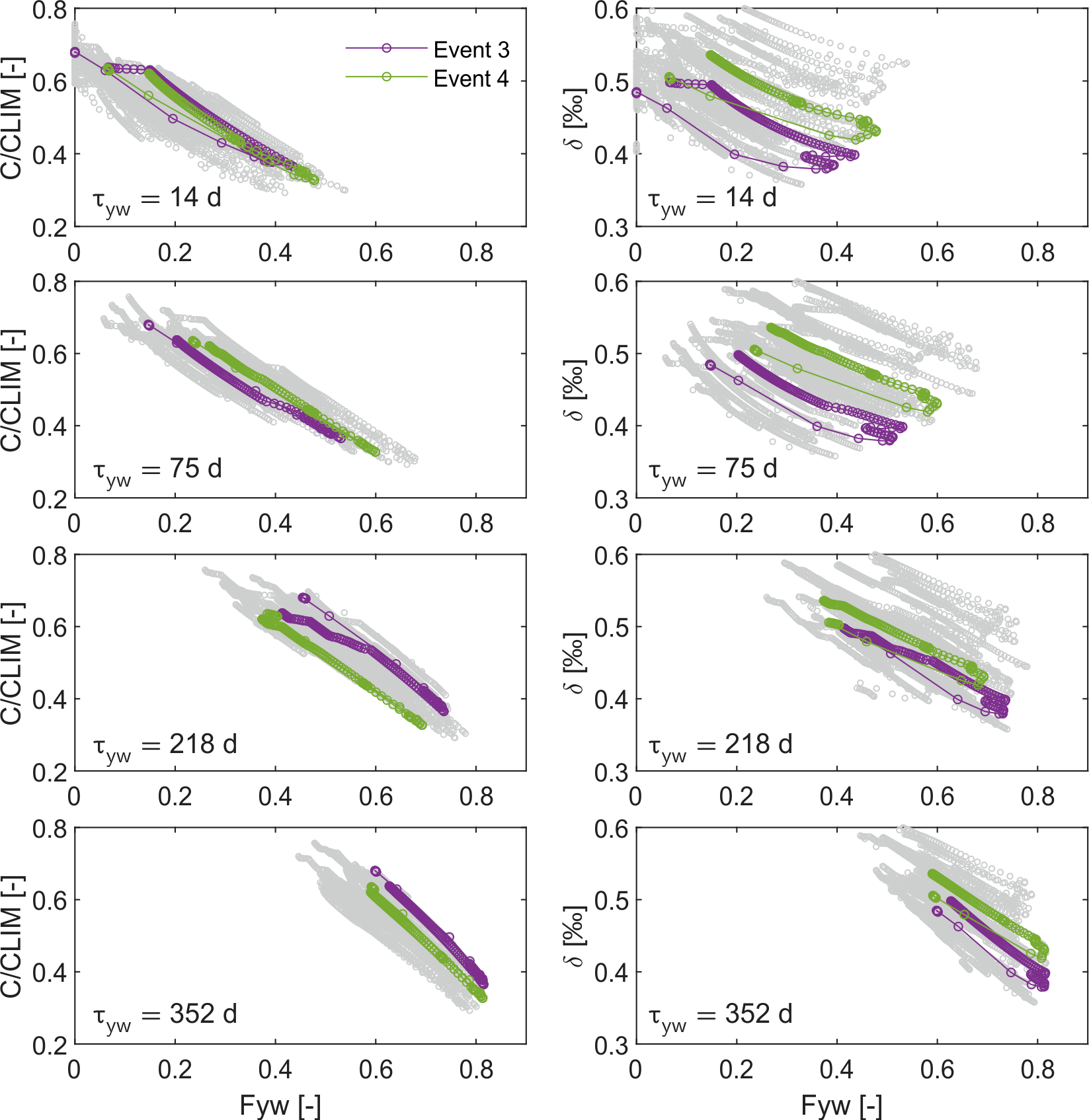
Clearly both $\text{SiO}_{2(\text{aq})}$ concentrations and $\delta$³⁰Si ratios produced by the simulation depend on the entire age distribution of the fluid. However, unlike our static fluid age distribution exercises (fig. 2), the age distributions derived from the SAS-function model are highly irregular. Hence it is not necessarily a given that the concentration or isotope ratio will demonstrate a clear trend as a function of some metric for fluid age. Yet, despite this irregularity, the fraction of water less than a given age F_yw, either computed from a model (Benettin, Bailey, et al., 2017) or from tracer cycle damping (Kirchner, 2016b) has been shown to serve as a reasonable predictor of system behavior. Timeseries of the various modeled F_yw are shown in Supplementary Information figure S5. Here we explore the extent to which fluid age can be correlated to $\text{SiO}_{2(\text{aq})}$ and/or $\delta$³⁰Si by extracting a range of young water fractions from the complete two-year simulation.

In each example, we define a unique value of age $\tau_{yw}$ which is considered “young” water as described in section 2.4. Beginning with $\tau_{yw}$ = 14 days, the fraction of fluid that falls at or below this value is never more than 50% (fig. 5). Relative to this very young water fraction, $C$/$C_{lim}$ shows a fairly clear linear relationship with a negative slope, meaning that when more of the water in the system is older than 14 days, the $\text{SiO}_{2(\text{aq})}$ concentration tends to be higher. This basic behavior is expected, yet the relationship is rather noisy ($r$² = 0.81). Events 3–4 (fig. 4A–B, described in Section 3.2) are once again highlighted. In particular, Event 3 still shows clear differences in $C$/$C_{LIM}$ in the rising and falling limb of the event even for the same value of fraction young water, suggesting that this fraction of the fluid age distribution is not a direct metric for the history of solute concentrations in the system.

Figure 5.(left column) $\mathbf{SiO_{2(aq)}}$ and (right column) $\delta$³⁰Si as a function of the young water fraction (F_yw). Four choices of the definition of “young” water are presented, including 14, 75, 218 and 352 days. Grey points indicate the entire 2-year dataset and are overlain by the two events selected in section 3.2.

The generally negative slope between $\text{SiO}_{2(\text{aq})}$ and fluid age fraction becomes clearer and more linear as we increase the definition of the age of young water to 75 days and higher. In each of these spaces, the overall two-year dataset is less scattered than in the 14-day example (F₇₅ $r$² = 0.85), and the two selected events presented in section 3.2 return fairly consistent values of $C$/$C_{LIM}$ for a given fraction of young water. Clearly the history of the system and the corresponding $\text{SiO}_{2(\text{aq})}$ concentrations prior to the start of a given event influence the absolute magnitude of $\text{SiO}_{2(\text{aq})}$ observed during a high discharge period. Yet from any given staring point, even for these highly irregular age distributions, the slope of decreasing $\text{SiO}_{2(\text{aq})}$ with increasing fraction of young water observed during a specific event is generally consistent across all events, reflecting the linear relationship between fluid age and solute concentration when $C$ << $C_{LIM}$ (eq 2, fig. 2). The result is that characteristic clockwise hysteretic loops observed in these solute concentrations as a function of discharge (fig. 4C & E) are produced by differences in the fluid age distribution across the rising and falling limbs of storm events.

In comparison to the $\text{SiO}_{2(\text{aq})}$ concentrations, the fluid $\delta$³⁰Si ratios are uniquely impacted by the restriction that solute concentrations less than the $C_{lim_{2}}$ value (150 µM) are associated with a non-fractionating reaction. Hence linearity between $\delta$³⁰Si and a very young water age fraction (e.g., ≤14 days) should be even less pronounced than the corresponding $\text{SiO}_{2(\text{aq})}$ relationship. This is consistent with the 2-year synthetic dataset, in which only a vague negative correlation is evident in the $\delta$³⁰Si values (fig. 5; F₁₄ $r$² = 0.16). Both events highlighted from section 3.2 show unique $\delta$³⁰Si values for the same fraction of young water across the rising and falling limbs of the storm hydrographs. This is clear even for Event 3, which showed very little distinction in $\delta$³⁰Si between the onset and recovery of the storm as a function of discharge (fig. 4D). Such behavior indicates that the component of water that is this young is not a good predictor of the corresponding $\delta$³⁰Si ratio of $\text{SiO}_{2(\text{aq})}$ in this system, and hence variation in the isotope ratios across a storm event are not reflecting the influence of this very young water.

As the definition of young water age is increased, the relationship to $\delta$³⁰Si remains quite irregular relative to the contemporaneous $\text{SiO}_{2(\text{aq})}$ - age behavior. The 2-year synthetic dataset of $\delta$³⁰Si vs. fluid age only really begins to condense into a compact linear relationship with negative slope when we approach young water age fractions of several hundred days (F₂₁₈ $r$² = 0.36; F₃₅₂ $r$² = 0.59). The individual events selected in section 3.2 continue to exhibit hysteretic loops more so than the corresponding $\text{SiO}_{2(\text{aq})}$ values, but these also tighten relative to the younger fluid age examples. In both Event 3 & 4, the rising limb of the hydrograph drives the system towards a larger fraction of young water in the system, and the fluid $\delta$³⁰Si ratios decrease, yet for the falling limb of the same event, the recovery in fluid $\delta$³⁰Si is generally more enriched, creating a counterclockwise pattern. This is despite very little difference in the $C$/$C_{LIM}$ values between the rising and falling limbs of the hydrographs when presented against the same fraction of young water metric.

Again, we caution that the underlying fluid age distributions at any given moment are highly irregular, yet it does appear that the $\text{SiO}_{2(\text{aq})}$ concentrations are easier to normalize to a given young water age fraction than their contemporaneous $\delta$³⁰Si ratios. In this particular synthetic system, the $\delta$³⁰Si ratios at a given value of F_yw during the recovery from a storm event are all consistently more enriched than during the onset of the storm, suggesting some consistency in the distinction between fluid age distributions across the rising and falling limbs of a given storm hydrograph that the concentrations are not sensitive to.

In total we observe a close correlation between $\text{SiO}_{2(\text{aq})}$ and fluid age across a broad definition of young water fractions. This relationship is not perfectly mimicked by the fluid $\delta$³⁰Si ratios. The distinction in behavior is a result of the restriction to fractionation only when the $C_{lim_{2}}$ threshold is exceeded, indicating that the stable isotope ratios of weathering-derived solutes are reflecting an older component of the fluid age distribution than contemporaneous concentrations. Hence a significant result of this study is that enrichment in the stable isotope signatures of solutes generated by weathering reactions reflect a component of the fluid age distribution that is distinct from that of the corresponding solute concentrations.

4.2. Sensitivity of fluid isotope signatures to watershed characteristics

Thus far we have developed a series of static models (section 3.1) and expanded to a single synthetic watershed in our extension to a SAS-function framework (section 3.2). From this basis clearly many parameter values could be subjected to sensitivity testing to explore the range of behavior anticipated in natural systems. Many seminal studies have considered the range of parameter space that encapsulate weathering reactions (e.g., Gaillardet et al., 1999; Helgeson et al., 1984; Lasaga et al., 1994; White & Blum, 1995; White & Brantley, 2003). In section 3.1 we relied upon such prior analysis taken from Maher (2010, 2011) and Torres and Baronas (2021) to define appropriate parameter values representative of silicate weathering reactions. Given this wealth of prior work, and notably the recent extensive Monte Carlo analysis of chemical parameterization explored by Torres and Baronas (2021), here we elect to focus on the sensitivity of the solutions to hydrologic parameterization of the SAS-function model. In what follows, we essentially hold chemistry (and isotopic fractionation) to a consistent behavior while exploring the effects of watershed and fluid age structural features on resultant solute concentrations and fluid isotope ratios. We return to consideration of chemical parameter variability in the subsequent sections.

The SAS-function framework is quite simple in the governing parameters that describe a given watershed (Rinaldo et al., 2015). The complexity of developing such a model for a real system lies in the necessity of historic datasets sufficient to allow spinup of the model, and the capacity to which such a simplified description can function as an appropriate representation of a given system. In our simulations, only three major parameters dictate the characteristics of fluid age distributions. These include the minimum and maximum “shape” parameters (z) for the SAS function and the “scale” parameter ($S_{0}$), jointly dictating how responsive a watershed is to perturbations (section 2.1). In comparison to our reference simulation (table 1), we consider two new sets of parameters. Set 1 (table 1) defines a system that is relatively small in comparison to our reference values (section 3.2). Set 2 is relatively larger in storage volume (and hence supports overall older fluid ages) and it has a larger variability in the “shape” parameter z. In total these three sets provide combinations of hydrologic parameters that produce realistic representations of natural watersheds ranging from small, flashy systems to larger dynamic systems all with a variety of reasonable representative shape factors for their fluid age distributions.

Both the solute concentrations and stable isotope ratios are significantly impacted by these choices of hydrologic parameterization (fig. 6). Comparison of these results to figure 4 produces sensible behavior, such that a larger system (fig. 6, red) supports generally older fluid ages and hence higher $\text{SiO}_{2(\text{aq})}$ concentrations. In contrast a smaller, flashy system (fig. 6, yellow) hosts shorter fluid residence times and hence overall lower solute concentrations. In all three representative watersheds, the selected storm event produces clockwise hysteresis loops in $\text{SiO}_{2(\text{aq})}$ as a function of discharge (fig. 6B). Additionally, the system with the large “scale” value hosting the oldest fluid ages and highest $\text{SiO}_{2(\text{aq})}$ concentrations is capable of producing the largest variation in $\text{SiO}_{2(\text{aq})}$ because it also has a broader variability in the “shape” parameter.

Figure 6.The same selected period of high discharge illustrated in figure 4 shown for the same reference parameters (blue) and now also for two more hydrologic parameter sets (table 1): Set 1 (yellow) and Set 2 (red). (A) event discharge values are plotted along the lower axis, while event precipitation is plotted along the upper axis. Concentrations are illustrated with solid lines, isotope ratios with open circles. (B) the corresponding $\mathbf{SiO_{2(aq)}}$ vs. discharge (Q) relationships, (C) $\delta$³⁰Si vs. Q. A red square indicates the start of each event in time, while a green diamond reflects the end of this high discharge period.

Similar comparison between figure 4 and figure 6 for the fluid $\delta$³⁰Si ratios is only impeded by the fact that the $\delta$³⁰Si y-axis scale is now much larger in the latter figure. The correspondingly higher $\text{SiO}_{2(\text{aq})}$ concentrations produced by the system with larger scale value and hence older fluid ages also creates much more enriched $\delta$³⁰Si ratios. The result is that in this system, which also spans a larger interval in the shape parameter, the sensitivity of $\delta$³⁰Si to discharge during storm events is much more pronounced (fig. 6C) and finally characteristic clockwise hysteresis patterns are discernible in the $\delta$³⁰Si-Q space. In contrast, the smaller catchment, though quite responsive in $\text{SiO}_{2(\text{aq})}$ as a function of discharge, shows essentially no variability at all in $\delta$³⁰Si-Q space across either storm. Though the absolute value of $\delta$³⁰Si is >0.0‰, the vast majority of fluid in this small system is too young to have crossed the $C_{lim_{2}}$ = 150µM threshold, and hence most of the fluid is not subject to a fractionating reaction.

It is important to remember that these three synthetic watersheds are all subjected to the same timeseries of precipitation and are required to produce the same discharge behavior over the two-year period. The result is that the same range and values of discharge are repeated across the three simulations. The distinction between them is then the characteristic age of fluid that is extracted from each system. For the relatively larger system with higher scale parameter, the fraction of fluid which is younger than some given age will thus be smaller than the same calculation for the smaller catchments with shorter overall fluid ages (section 4.1).

Figure 7.Two years of simulated discharge, solute concentrations and isotope ratios for three different hydrologic parameter sets (table 1): reference (blue), Set 1 (yellow), Set 2 (red). (A) The fraction of fluid younger than ∼200 days vs. discharge, (B) $\mathbf{SiO_{2(aq)}}$ vs. the same metric for fraction of young fluid, and (C) $\delta$³⁰Si vs. the same fraction of young fluid.

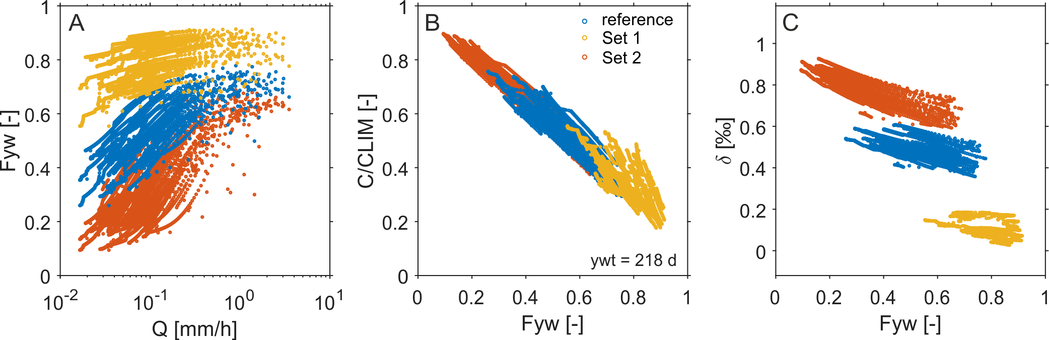
Using a metric for young water age of ~200 days, the three watersheds are clearly distinct in the fraction of fluid less than or equal to this value over the full 2-year simulation (fig. 7A). The corresponding $\text{SiO}_{2(\text{aq})}$ concentrations produced from these watersheds are then linearly related to this fraction of young fluid and delineate a clear trend in which the watershed with the largest scale parameter produces the highest concentrations (fig. 7B). Once again, much of the variability in concentrations of weathering-derived solutes such as $\text{SiO}_{2(\text{aq})}$ as a function of discharge can be resolved through the direct relationship between concentration and fluid age. Further, these three watersheds produce $C$/$C_{LIM}$ values that overlap with one another at various points in time when each watershed is hosting characteristically younger or older fluid ages relative to their own average value.

In contrast, fluid $\delta$³⁰Si ratios remain highly distinct from one another in each of these systems and very rarely overlap with one another at all across the complete 2-year simulations (fig. 7C). Clearly the fraction of young water produced by a given watershed does not map onto a linear relationship with fluid $\delta$³⁰Si enrichment in the same way as the corresponding $\text{SiO}_{2(\text{aq})}$ concentrations. Instead, the same value of fraction young water produces very different $\delta$³⁰Si values depending upon the size and structure of a given watershed. While storm events can and do exert influence on the resultant $\delta$-Q relationship of fluids draining watersheds (section 4.1), the absolute magnitude of the isotope ratios of solutes subject to fractionating weathering reactions are largely predicated on the overall component of the fluid age distribution that allows fractionation (fig. 5). This age component is tied to the characteristic storage volume and functional form of the fluid age distribution in a given system more so than the transient effects of storm events. Furthermore, the discontinuity introduced by a reaction that only fractionates above a specific solute concentration (eq 14) undermines the emergence of a continuous relationship between fluid age and $\delta$³⁰Si across these non-uniform systems. This leads to a second important inference derived from our model-driven study, that relative to solute concentrations and in the absence of changes in the chemical parameters driving weathering reactions, the absolute magnitude of fluid isotope fractionation in geogenic solutes appears to be dictated by the structure and storage of a given watershed more so than transient events that perturb the system.

4.3. Revisiting common models for fractionation

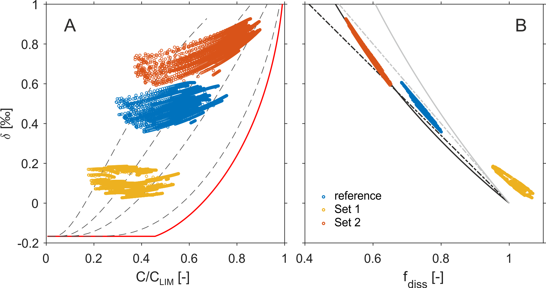
Having considered the relationship between isotope ratio and fluid age, which leads to a deeper understanding of the factors that set the range of delta values observed in a given system, we now revisit more common models used to relate isotopic fractionation to solute concentrations in natural watersheds. Such approaches would typically begin by directly relating isotope ratios to solute concentration (fig. 8A). Using the simpler results of Section 3.1 as a reference point, the SAS model simulations are consistently distinct from the batch model, and largely remain associated with gamma distributions of shape factor 1.0 or less.

Figure 8.(A) The same solution space produced in figure 2C now with the 2 years of SAS-function model output overlaid from hydrologic parameter sets 1 (yellow), 2 (red) and reference (blue) as described in table 1. The results from the uniform age model (red solid line) and gamma distributions (dashed lines) are detailed in section 3.1. (B) 2 years of tran-SAS model output for the three parameter sets (table 1) plotted as the fraction of $\mathbf{SiO_{2(aq)}}$ remaining in solution relative to what would be found if no clays had formed (f_diss). Rayleigh (solid black line) and steady-state open flow-through (dashed black line) models are fit to these data from a starting point of f_diss = 1 and $\delta$³⁰Si = 0.0‰. Rayleigh (solid gray line) and steady-state open flow-through (dashed gray line) models use the intrinsic $\alpha$₂ = 0.998 embedded within the SAS-function model simulations for the formation of new secondary clays.

Fluid $\delta$³⁰Si values are often cast against some metric of reaction progress in order to infer a fractionation factor in natural systems, for example using a simplified application of the Rayleigh equation (e.g., Baronas et al., 2018; Dellinger et al., 2015; Georg et al., 2007; Tipper et al., 2012). If we were to use $C$/$C_{LIM}$ as this metric, it becomes apparent that fitting such a simple model to one of these datasets could foster significant misinterpretation of the underlying system. The tran-SAS derived data are generally quite enriched relative to the batch model, and yet the classic exponential enrichment in isotope ratio with reaction progress is strongly muted, leading to a clustering of the $\delta$³⁰Si ratios in a narrow range despite relatively large variations in solute concentration. This capacity for enrichment even at small values of $C$/$C_{LIM}$ (fig. 2C) is tied to a dampening in the extent to which isotopic enrichment can further develop (fig. 2B) is thus a hallmark of isotopic signatures in fluid age distributions featuring predominantly young water with a long tail, such as the gamma distribution. This behavior is not immediately suited to application of such simple models for fractionation and requires further treatment to evaluate appropriately.

Turning to a better metric for the $\text{SiO}_{2(\text{aq})}$ lost from solution, we calculate the ratio of silicon to some geogenic element which is not incorporated into secondary minerals or biologically cycled (e.g., Charbonnier et al., 2020; Fernandez et al., 2022). For example, using the silicon/sodium (Si/Na) ratio of the bedrock or primary mineral assemblage as a reference point, the corresponding Si/Na of the fluid may then be corrected to a fraction dissolved (f_diss) that is the component of silicon that remains in the fluid after the influence of secondary mineral formation and vegetation cycling. In the present model, we can constrain a similar f_diss metric simply by running the model in the absence of any secondary clay formation and taking the ratio of $\text{SiO}_{2(\text{aq})}$ to this non-precipitating concentration (fig. 8B). As expected, we find that some of the $\text{SiO}_{2(\text{aq})}$ that would have appeared in solution due to the dissolution of primary minerals has been lost as a result of the formation of secondary clays in parameter set 2 and our reference case (table 1). For parameter set 1, the majority of fluid is so young that it remains below the $C_{lim_{2}}$ threshold, and hence both the primary minerals and secondary clay are dissolving. In this example, the f_diss calculation returns a value slightly >1, as would be expected if the Si/Na_bedrock correction were applied to a real-world dataset featuring this behavior (e.g., Fernandez et al., 2022).

The result is a much tighter clustering of the data into a narrow range of values, highlighting the utility of this f_diss normalization. Again, considering common models for fractionation, first, a classic Rayleigh distillation model can be fit to the data using a starting point of f_diss = 1 and $\delta$³⁰Si = 0.0‰. This calculation does particularly well in recovering the complete 2-year simulation for parameter set 2 (table 1) using a fractionation factor of $\alpha$ = 0.9986 or $\epsilon$ = 1.4‰ (fig. 8B). A second model framework commonly used in application to weathering systems is the steady-state open flow-through relationship developed by Bouchez et al. (2013), which is essentially another version of isotopic mass balance. For this model, a single value of $\alpha$ does not describe the complete 2-year dataset from parameter set 2, but it may be bounded between $\alpha$ values of 0.998 (2.0‰) and 0.9983 (1.7‰).

Given our underlying chemical parameterization (table 1), we recognize that both of these models are challenged in producing appropriate representations of the relationship between $\delta$³⁰Si and f_diss. In the Rayleigh model, we lack representation of the continuing contribution of $\text{SiO}_{2(\text{aq})}$ with $\delta$³⁰Si = 0.0‰ to solution due to primary mineral dissolution. In the Bouchez et al. (2013) approach, the calculation essentially subtracts fractionating effects from a bedrock value at steady state, while in these simulations there is no point across the entire 2-year record (fig. 3) where concentrations or isotope ratios could be considered stable in time. Here, each simulation would need to be fit with a different fractionation factor regardless of whether the Rayleigh or steady-state open flow-through frameworks are chosen. Finally, parameter set 1 is impossible to treat in either framework because of the effect of secondary clay dissolution in the calculation of f_diss.

Both simplified models (fig. 8B) return fractionation factors that are smaller (i.e., closer to 1.0) than the imposed $\alpha_2$ = 0.998 value embedded in the SAS-function model, as expected for field scale measurements relative to those constrained under batch reaction conditions (Druhan et al., 2019; Druhan & Maher, 2017; Golla et al., 2021). One means of reconciling this disparity that is consistent with our SAS framework is the possibility of combining simple fractionation models with equally simple representations of static fluid age distributions. Clearly even the use of a time-invariant fluid age distribution such as the gamma functions shown in figure 8A offers a much closer representation of these SAS-function results than the corresponding uniform-age batch model. While significant data and model development are necessary to produce an accurate SAS-function model for a given catchment, these simpler representations of fluid age distributions are relatively easy to work with and have already been applied to weathering reactions (Ibarra et al., 2017; Maher, 2011; Maher & Chamberlain, 2014) and to a lesser extent isotopic fractionation (Druhan & Maher, 2017; Fernandez et al., 2022). If only uniform fluid age is considered, then common models relating fractionation to reaction progress can appear to function correctly despite inappropriate underlying assumptions and for inaccurate parameter values. Hence another key result of our work is to emphasize the necessity of convolving even the most basic models for fractionation with reasonable representations of fluid age distribution when interpreting the stable isotope signatures of weathering reactions in solutes draining from watersheds.

4.4. Comparison to real-world observations

Riverine solute stable isotope signatures are broadly used as a means of unpacking the origins and cycling of geogenic elements in watersheds as they are nominally unaffected by dilution and are only fractionated by a subset of weathering reactions (Charbonnier et al., 2020, 2022; Dellinger et al., 2015; Engström et al., 2010; Ercolani et al., 2019; Fernandez et al., 2022; Frings et al., 2016; Georg et al., 2006; Henchiri et al., 2016; M. Y. H. Li et al., 2021; Pogge von Strandmann et al., 2008; Pogge von Strandmann & Henderson, 2015; Pokrovsky et al., 2013; Riotte et al., 2018). In recent years, increasingly high frequency solute datasets have been produced in an effort to detail the relationships between weathering-derived solutes and fluid drainage through landscapes (Floury et al., 2017; Rode et al., 2016; von Freyberg et al., 2017). In tandem, high resolution isotopic datasets are being developed for these solutes, including a very recent compilation of $\delta$³⁰Si in six low order streams located across a wide variety of landscapes, climates and ecosystems (Fernandez et al., 2022). In each of these systems, $\text{SiO}_{2(\text{aq})}$ and $\delta$³⁰Si timeseries were recorded during a major storm event. Only one of these watersheds currently has a SAS-function type hydrologic model developed specifically for it (Visser et al., 2019), and unfortunately the model was constructed for a different subcatchment than the Fernandez et al. (2022) study, yet in total the six sites offer an important opportunity to contextualize the results of our model development. In turn, our work offers a foundation for the interpretation of these emerging datasets and creates a quantitative framework from which to draw hypotheses for the observations recorded in natural systems.

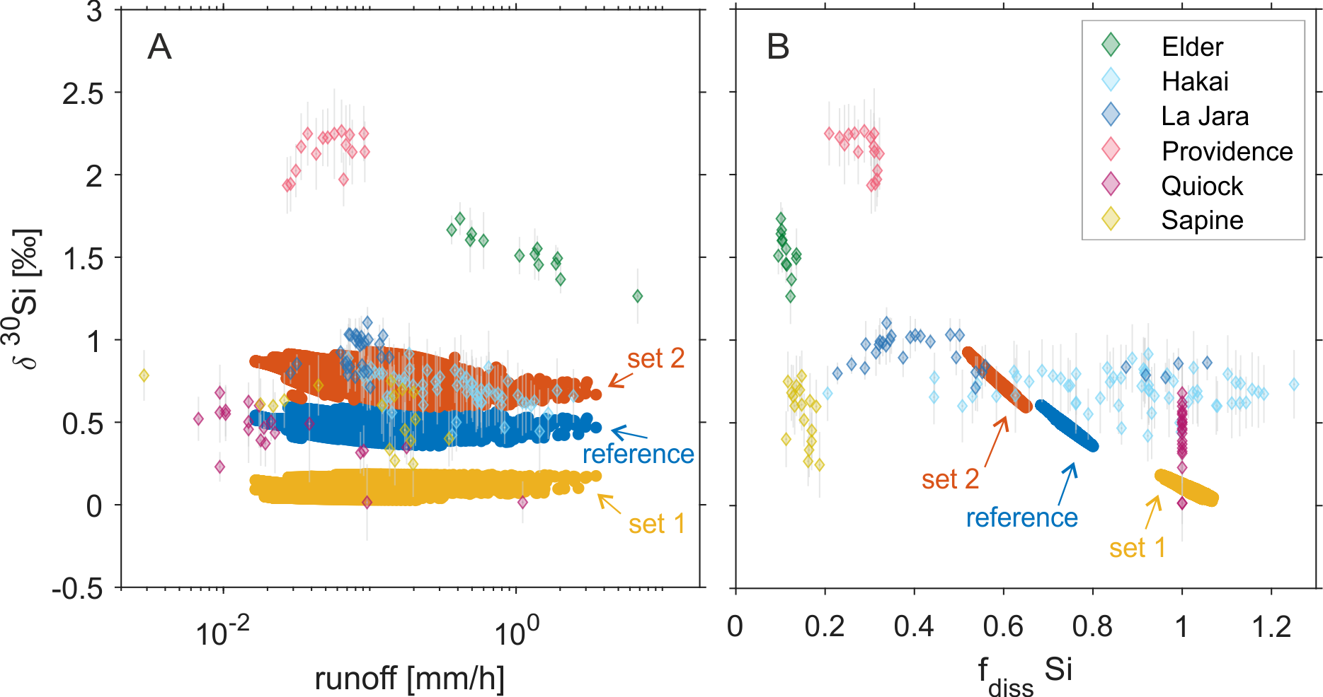
Four of the six low order streams are located on continental mainlands, including Sapine (Mont-Lozère, France), La Jara (New Mexico, USA), Providence (California, USA) and Elder (California, USA). The remaining two are positioned on islands, including Hakai (Calvert Island, British Colombia, Canada) and Quiock (Basse-Terre, Guadeloup, France). The details of these sites, the storms that were sampled, and the analytical methods for $\text{SiO}_{2(\text{aq})}$ and $\delta$³⁰Si are all provided in Fernandez et al. (2022). Here, we simply note that in total, the runoff recorded across the storms spanned over four orders of magnitude and that the range of runoff rates recorded for any given site are largely predicated on the duration and intensity of the storm event rather than the physical characteristics of the catchment. Our synthetic watersheds were run over a comparable range of discharge rates, and in general these three “systems” (table 1) act as an additional three datasets in the compilation (fig. 9A).

Figure 9.Stream solute $\delta$³⁰Si ratios measured in six low order catchments spread across the world (Fernandez et al., 2022), compared with the output from our three watershed parameter sets (table 1). (A) $\delta$³⁰Si (A) as a function of runoff and (B) as a function of f_diss as defined in section 4.3. All $\delta$³⁰Si values reported by Fernandez et al. (2022) are normalized to their respective bedrock values, allowing a direct comparison to our modeled $\delta$³⁰Si values with bedrock $\delta$³⁰Si = 0.0‰.

It is imperative that we qualify the diversity of unique lithologies, climates, and weathering intensities represented by these six catchments. In contrast, the geochemical parameterization of our model is single component, and builds upon that developed by Maher (2010, 2011) (Supplementary Section S5), which was originally based on a multi-component numerical model of the soil chronosequence located near Santa Cruz, California, USA (Supplementary Information S4). This earlier model (Maher et al., 2009) allowed a relatively significant amount of kaolinite development, and hence our parameters are generally most appropriate to systems experiencing a relatively high degree of weathering intensity. Some of the watersheds reported in Fernandez et al. (2022) exhibit even more advanced weathering (e.g., Quiock), while others show far less (e.g., Providence). In keeping with the approach of Maher (2010, 2011) we compare our model results to this wide diversity of catchments, recognizing the fact that the weathering intensity and secondary clay assemblage of each system will influence the values of ${k}_{eff}$ and $C_{LIM}$ appropriate to these locations (Ackerer et al., 2018, 2021). It is the purpose of this study to provide a generalized framework and draw broad comparison to a diversity of natural systems, while future studies can and should develop more site-specific parameterization appropriate to individual watersheds of interest. What we present here is intended to motivate exploration of the extent to which geochemical composition of individual sites and heterogeneity of mineral assemblages therein manifest in event-scale $C$-$\delta$-Q dynamics.

Given these qualifications, and for a comparable range of runoff values, the SAS-function-based model results are quite consistent and generally fall into the same range of $\delta$³⁰Si as the natural watersheds (fig. 9A). We note that all $\delta$³⁰Si values reported for the natural systems are given as the difference between the stream $\delta$³⁰Si ratios and the bedrock $\delta$³⁰Si ratio characteristic of each site (i.e., ∆³⁰Si) and are thus directly comparable to our synthetic values. Generally, in this solution space, it is difficult to distinguish unique behavior among many of the catchments. For example, La Jara and Hakai both closely overlap with our synthetic model results and would seem comparable despite the fact that the former is a high elevation, semi-arid continental site hosting a mixed conifer forest and the latter is a low elevation coastal temperate rainforest.

Clear distinctions between the six field sites and three synthetic watersheds are revealed when the data are recast in terms of the f_diss metric for $\text{SiO}_{2(\text{aq})}$ remaining in solution (fig. 9B). For the natural systems, this is done using the Si/Na_bedrock ratio characteristic of each site (Fernandez et al., 2022) while for our model results it is accomplished as described in section 4.3. In this space, each field site tightly clusters to itself, despite the similarity in runoff rates. As described in section 4.2, our model results also distinguish between each of the three hydrologic parameter sets tested (table 1) and fall on a general trajectory that is consistent with the natural systems. For f_diss near 1.0, $\delta$³⁰Si ratios are low, and as more $\text{SiO}_{2(\text{aq})}$ is lost from solution due to the effects of secondary clay formation and vegetation cycling, $\delta$³⁰Si ratios become enriched. Notably the two island sites (Hakai and Quiock) both return f_diss $\geq$ 1.0, similar to the synthetic results for parameter set 1 (table 1). As discussed in Fernandez et al. (2022) these two sites are heavily weathered and are exporting essentially all of the $\text{SiO}_{2(\text{aq})}$ that is dissolved from bedrock, consistent with our model behavior. Furthermore, Fernandez et al. (2022) were challenged to offer an explanation for the low but consistent apparent enrichment in stream $\delta$³⁰Si ratios in these sites despite f_diss ≥ 1.0. While our synthetic data are not as enriched as these natural sites, the model offers a plausible explanation in that some component of the fluid arriving in the streams at these sites must be old enough to have reached solute concentrations that support secondary clay formation and hence elevated the $\delta$³⁰Si values above bedrock.

In the remaining continental sites, Fernandez et al. (2022) note the clustering of data specific to each location and suggested that the unique structure and functioning of each watershed is a primary control on the resultant $\delta$³⁰Si signatures. Our merging of a SAS-function with fractionating weathering reactions now provides a quantitative model framework which confirms this inference. As demonstrated above (fig. 7C) the relationship between fluid age and dissolved solute $\delta$³⁰Si ratios is not as straightforward as that of $\text{SiO}_{2(\text{aq})}$. Rather, the unique structure, storage and fluid age distribution functions of a given watershed are the primary factors setting the observed enrichment in riverine $\delta$³⁰Si values even as the system is overprinted by transient storm events. This structure-based differentiation is also reflected in the natural systems that support fractionation (fig. 9B), however, there is no simple mapping between the $\delta$³⁰Si values characteristic of a given site and any single physical metric. For example, Elder drains the largest basin area of the six sites, yet Providence exhibits the largest isotopic enrichment. Rather, the extent to which each of these systems can produce its own signature range of isotopic enrichment in solutes impacted by weathering reactions may offer a clearer indicator of the storage and age distribution characteristics of a given watershed than these physical parameters.

Finally, we note that Fernandez et al. (2022) considered the capacity for each of these sites to host a unique suite of weathering reactions and vegetation effects, ultimately producing unique chemical and isotopic parameterization. This variability has been held constant in the present study to focus on the manifestation of hydrologic characteristics in $C$-Q and $\delta$-Q behavior. Were we to open this particular version of “Pandora’s box”, we expect that the models could recover a larger range of f_diss and $\delta$³⁰Si and hence more overlap with the observations reported for these natural watersheds. Furthermore, we recognize that the SAS-function model results shown here were based on a common spinup period and a common two-year simulation which forced all three synthetic watersheds to produce the same discharge values (fig. 7A). None of the natural watersheds shown here reflect these synthetic data and creating a calibrated SAS-function model for any of these systems constitutes a significant effort (e.g., Visser et al., 2019). Given these challenges, we offer the present synthetic analysis as a reference point, using three descriptions of low order watersheds (table 1) that are realistic, and subjecting them to a two-year simulation that is representative of inputs and discharge behavior in many natural systems. In doing so we offer a quantitative analysis of the extent to which differences in hydrologic structure and the routing of water through landscapes impact the observed signatures of weathering in the solutes that drain from these landscapes. Holding all other factors constant, we have shown that the observed fractionation in isotope ratios caused by weathering reactions is easily differentiated among these systems. We conclude that the stable isotope ratios of weathering-derived solutes draining from low order watersheds are predicated on the characteristic age distribution of the fluid these systems host, more so than transient perturbations. Hence large variations in isotopic enrichment observed for a given location are likely associated with alterations in the reactive pathways that mobilize and cycle these solutes, or with fundamental changes in the routing of water to the stream.

5. Conclusions

Basic relationships between reaction rate and flow rate have existed in the chemical engineering literature for decades. In application to weathering reactions in Critical Zone environments this fundamental balance has largely been considered in relation to long-term monitoring of riverine solute fluxes and hence leveraged static representations of both reactivity and fluid age distributions. Now, novel monitoring and analytical techniques are facilitating increasingly high resolution spateotemporal tracking of solute flux and discharge, in tandem with advances in metaloid isotope ratios as fingerprints of specific reactive pathways within these complex systems. The inevitable result is that steady state assumptions are becoming increasingly limiting, and hence models capable of honoring the dynamic nature by which infiltration is delivered to and routed through the Critical Zone are needed.

This study reports the development of such a model that, for the first time, merges the effects of chemical weathering, fractionating reactions and transient fluid age distributions in one coherent simulation. Based on this advancement, we have shown that the isotope ratios of geogenic solutes can produce hysteresis patterns as a function of discharge during precipitation events, leading to a new conceptualization of $C$-$\delta$-Q relationships. However, these isotope ratios do not simply mirror associated $C$-Q behavior. Rather, the necessity to cross secondary mineral solubility thresholds prior to fractionation creates a discontinuity in the behavior of $C$ and $\delta$ in these systems, ultimately causing the isotope ratios to vary less over individual storm events than their corresponding solute concentrations. This discontinuity causes the isotope ratios to differentiate more as a result of differences in the physical characteristics describing the storage size and fluid age distributions supported by a given catchment. The result is that, if all other factors are held constant, the isotope ratios measured in two systems with distinct structures and fluid age distributions should be quite disparate. This conclusion appears to be in agreement with a novel dataset of $\delta$³⁰Si measured during storm events in six low-order streams located across the globe.

Clearly $\delta$³⁰Si ratios recorded across storm hydrographs offer a novel means of analyzing weathering reactions and $C$-Q relationships in critical zone environments (Fernandez et al., 2022). We note here that we have used $\delta$³⁰Si only as an example that is rich with potential when coupled to a hydrologic model that resolves the fluid age balance of water stored in a catchment. One could easily recast this framework to any number of stable isotope systems for rock-derived elements which exhibit mass-dependent fractionation due to incongruent weathering.

ACKNOWLEDGEMENTS

JLD acknowledges funding support from the U.S. National Science Foundation NSF-EAR-2135405. PB thanks ENAC school at EPFL for financial support. Both authors wish to thank Ciaran Harman and two anonymous reviewers for their valuable feedback, as well as Julien Bouchez, Jotis Baronas and the IPGP “$\delta$-Q working group” for constructive feedback during the development of this study.

SUPPLEMENTARY INFORMATION

https://doi.org/10.5281/zenodo.8211494

DATA AVAILABILITY STATEMENT

The data and code associated with this paper can be found in Benettin and Druhan (2023). Stream chemistry data in figure 9 comes from Fernandez et al. (2022).

Editor: Mark Brandon, Associate Editor: Daniel Ibarra